Simple Linear Regression: OLS Derivation Explained

This tutorial explains the mathematical foundation of Simple Linear Regression and shows how the famous formulas for the slope (m) and intercept (b) are derived. Rather than treating the formulas as magic, we will build them step by step from first principles and understand why the algorithm works. The source material focuses on deriving the Ordinary Least Squares (OLS) solution and understanding the loss function that drives Linear Regression.

Introduction

When we first learn Linear Regression, the algorithm often looks deceptively simple. We are given a set of data points and are told that the goal is to draw a line that best represents the relationship between the input variable and the output variable.

Consider a dataset where:

• Input (X) = CGPA
• Output (Y) = Salary Package

As CGPA increases, the package generally increases as well. However, real-world data is rarely perfectly linear. The points are usually scattered around an imaginary trend line rather than lying exactly on it. Because of this imperfection, we need a method that can find the line that represents the data as accurately as possible.

The question therefore becomes:

How do we find the best line among infinitely many possible lines?

That is exactly what Linear Regression solves.

Recap: The Equation of a Straight Line

The equation of a straight line is:

$$y=mx+b$$

Where:

• m represents the slope of the line.
• b represents the intercept.
• x is the input feature.
• y is the predicted output.

In the CGPA-package example:

• x = CGPA
• y = Predicted Package

Once we know the values of m and b, we can predict the package for any CGPA value. Therefore, the entire problem of Linear Regression can be reduced to one simple objective: Find the correct values of m and b.

What Makes a Line "Best"?

Imagine several different lines passing through the same dataset. Some lines may pass far away from most points. Some lines may pass through a few points but miss many others.

The ideal line is the one that stays as close as possible to all points collectively. The objective is not necessarily to pass through every point. In real-world datasets that is usually impossible. Instead, the goal is to minimize the overall prediction error across all observations. This leads us to the concept of error.

Understanding Prediction Error

Suppose a student's actual package is $Y_i$ and our regression line predicts $\hat{Y_i}$. ​ The difference between them is the prediction error:

$$Error = Y_i - \hat{Y_i}$$

If:

• Aactual Package = 8 LPA
• Predicted Package = 7 LPA

Then:

$$Error=1$$

Similarly, if:

• Actual Package = 7 LPA
• Predicted Package = 8 LPA

Then:

$$Error=−1$$

The error tells us how much our prediction differs from reality.

Why We Cannot Simply Add Errors

A natural idea would be:

$$Total Error=e_1+e_2+e_3+...+e_n$$

Unfortunately, this does not work. Positive and negative errors cancel each other. For example:

$$(+10)+(−10)=0$$

A total error of zero might suggest perfect predictions even though every prediction could be wrong. Therefore, we need a better measurement.

Squaring the Errors

To avoid cancellation, we square every error.

$$e_i^2$$

​ This provides two major benefits.

Benefit 1: All Values Become Positive

Whether the error is positive or negative, squaring makes it positive.

$$(-5)^2=25 \\ (5)^2=25$$

No cancellation occurs.

Benefit 2: Large Mistakes Are Penalized More

Consider:

• Error = 2 → Squared Error = 4
• Error = 10 → Squared Error = 100

Large mistakes receive a much larger penalty. This encourages the algorithm to avoid predictions that are extremely far from the actual values.

Building the Loss Function

If we square every error and add them together, we obtain:

$$L=e_1^2​+e_2^2​+e_3^2​+⋯+e_n^2​$$

Using summation notation:

$$L=\sum_{i=1}^{n}e_i^2$$

This quantity is called the Loss Function or Cost Function in machine learning. The purpose of Linear Regression is now very clear:

Find the values of m and b that make this loss function as small as possible.

Replacing Error with Actual and Predicted Values

We know:

$$e_i = Y_i - \hat{Y_i}$$

Substituting into the loss function:

$$L=\sum_{i=1}^{n}(Y_i-\hat{Y_i})^2$$

This expression measures the total squared prediction error across the dataset.

Introducing the Line Equation

Our prediction comes from the line:

$$\hat{Y_i} = mX_i + b$$

Substituting into the loss function:

$$L=\sum_{i=1}^{n}(Y_i-(mX_i+b))^2$$

This is one of the most important equations in Linear Regression. Notice something crucial, the values $X_i$ and $Y_i$ come from the dataset and are fixed. The only unknowns are m and b. Therefore:

$$L=f(m,b)$$

The loss function depends entirely on the slope and intercept.

Visualizing the Optimization Problem

To understand how Linear Regression finds the best-fit line, it is helpful to think about what happens when we change the values of the slope (m) and intercept (b). Every possible combination of these two parameters produces a different line, and each line results in a different amount of prediction error.

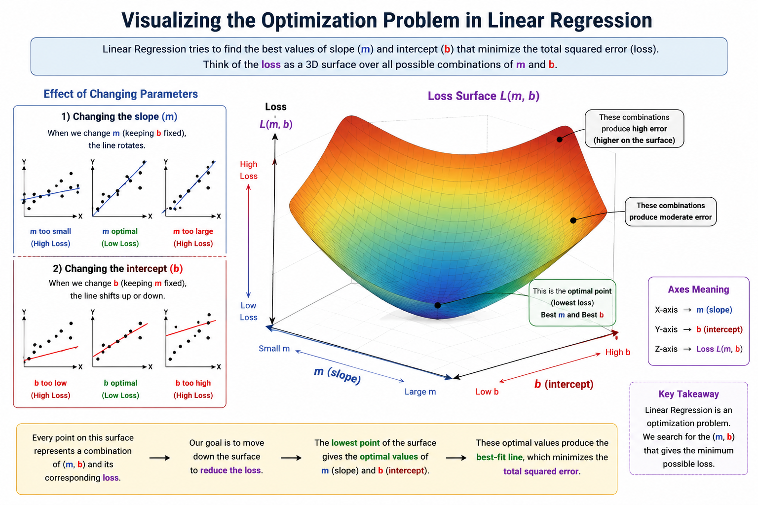
When the value of m changes while b remains fixed, the line rotates around its intercept. Some rotations bring the line closer to the data points and therefore reduce the overall error, while other rotations move the line away from the data and increase the error. In a similar way, changing the value of b shifts the entire line upward or downward without altering its slope. Depending on how well the shifted line aligns with the data, the prediction error may either decrease or increase.

Since both m and b directly affect the prediction error, the loss function can be viewed as a function of two variables. A useful way to visualize this relationship is through a three-dimensional graph in which:

• The X-axis represents the slope (m)
• The Y-axis represents the intercept (b)
• The Z-axis represents the loss value

Rather than appearing as a flat surface, this graph typically resembles a large bowl-shaped valley. Every point on the surface corresponds to a particular combination of slope and intercept, and the height of that point indicates how much error is produced by that combination. Parameter values that generate large prediction errors appear higher on the surface, while parameter values that produce smaller errors appear lower.

At the very bottom of this valley lies a special point that corresponds to the optimal values of m and b. This point represents the combination of slope and intercept that minimizes the loss function, making it the best-fit line for the dataset. The entire objective of Linear Regression is therefore to locate this lowest point on the error surface and use the corresponding parameter values to construct the final prediction model.

How Do We Find the Minimum?

In calculus, a minimum point occurs where the derivative becomes zero.

For functions of a single variable:

$$\frac{\partial L}{\partial x} = 0$$

However, our loss function depends on two variables:

• m
• b

Therefore, we must use partial derivatives.

We compute:

$$\frac{\partial L}{\partial m} = 0$$

and

$$\frac{\partial L}{\partial b} = 0$$

Solving these two equations simultaneously gives us the optimal values of m and b.

Deriving the Intercept Formula

At this point, our objective is to minimize the loss function:

$$L = \sum_{i=1}^{n}(Y_i - (mX_i + b))^2$$

Since the loss function depends on both m and b, we need to calculate partial derivatives. Let us first derive the formula for the intercept b. We begin by taking the partial derivative of the loss function with respect to b and setting it equal to zero.

$$\frac{\partial L}{\partial b} = 0$$

Starting with:

$$L = \sum_{i=1}^{n}(Y_i - (mX_i + b))^2$$

Applying differentiation:

$$\frac{\partial L}{\partial b} = \sum_{i=1}^{n} 2(Y_i-(mX_i+b))(-1)$$

Factoring out constants:

$$\frac{\partial L}{\partial b} = -2 \sum_{i=1}^{n} (Y_i-mX_i-b)$$

Setting the derivative equal to zero:

$$-2 \sum_{i=1}^{n} (Y_i-mX_i-b) = 0$$

Dividing both sides by -2:

$$\sum_{i=1}^{n} (Y_i-mX_i-b) = 0$$

Expanding the summation:

$$\sum_{i=1}^{n}Y_i - m\sum_{i=1}^{n}X_i - \sum_{i=1}^{n}b = 0$$

Since b is a constant:

$$\sum_{i=1}^{n}b = nb$$

Substituting:

$$\sum_{i=1}^{n}Y_i - m\sum_{i=1}^{n}X_i - nb = 0$$

Moving terms:

$$nb = \sum_{i=1}^{n}Y_i - m\sum_{i=1}^{n}X_i$$

Dividing by n:

$$b = \frac{\sum_{i=1}^{n}Y_i}{n} - m \frac{\sum_{i=1}^{n}X_i}{n}$$

Recall the definitions of the means:

$$\bar{Y} = \frac{\sum_{i=1}^{n}Y_i}{n}$$ $$\bar{X} = \frac{\sum_{i=1}^{n}X_i}{n}$$

Substituting these values:

$$b = \bar{Y} - m\bar{X}$$

Therefore, the intercept formula becomes:

$$b = \bar{Y} - m\bar{X}$$

Deriving the Slope Formula

Now let us derive the formula for the slope m. We again start with the loss function:

$$L = \sum_{i=1}^{n}(Y_i - (mX_i + b))^2$$

Taking the partial derivative with respect to m:

$$\frac{\partial L}{\partial m} = 0$$

Applying the chain rule:

$$\frac{\partial L}{\partial m} = \sum_{i=1}^{n} 2(Y_i-(mX_i+b)) (-X_i)$$

Factoring out constants:

$$-2 \sum_{i=1}^{n} X_i(Y_i-(mX_i+b)) = 0$$

Dividing both sides by -2:

$$\sum_{i=1}^{n} X_i(Y_i-(mX_i+b)) = 0$$

Expanding:

$$\sum_{i=1}^{n}X_iY_i - m\sum_{i=1}^{n}X_i^2 - b\sum_{i=1}^{n}X_i = 0$$

Rearranging:

$$m\sum_{i=1}^{n}X_i^2 = \sum_{i=1}^{n}X_iY_i - b\sum_{i=1}^{n}X_i$$

Substituting:

$$b = \bar{Y} - m\bar{X}$$

gives:

$$m\sum_{i=1}^{n}X_i^2 = \sum_{i=1}^{n}X_iY_i - (\bar{Y}-m\bar{X}) \sum_{i=1}^{n}X_i$$

Expanding:

$$m\sum_{i=1}^{n}X_i^2 = \sum_{i=1}^{n}X_iY_i - \bar{Y}\sum_{i=1}^{n}X_i + m\bar{X}\sum_{i=1}^{n}X_i$$

Collecting all terms containing m:

$$m\sum_{i=1}^{n}X_i^2 - m\bar{X}\sum_{i=1}^{n}X_i = \sum_{i=1}^{n}X_iY_i - \bar{Y}\sum_{i=1}^{n}X_i$$

Factoring out m:

$$m \left( \sum_{i=1}^{n}X_i^2 - \bar{X}\sum_{i=1}^{n}X_i \right) = \sum_{i=1}^{n}X_iY_i - \bar{Y}\sum_{i=1}^{n}X_i$$

Solving for m:

$$m = \frac{ \sum_{i=1}^{n}X_iY_i - \bar{Y}\sum_{i=1}^{n}X_i }{ \sum_{i=1}^{n}X_i^2 - \bar{X}\sum_{i=1}^{n}X_i }$$

This is the first form of the slope equation.

After algebraic simplification, it can be rewritten as:

$$m = \frac{ \sum_{i=1}^{n} (X_i-\bar{X}) (Y_i-\bar{Y}) }{ \sum_{i=1}^{n} (X_i-\bar{X})^2 }$$

This is the final Ordinary Least Squares (OLS) slope formula that is commonly found in textbooks and machine learning libraries.

OLS vs Gradient Descent

At this stage, we have successfully derived mathematical formulas for the slope (m) and intercept (b) using calculus. These formulas allow us to directly calculate the parameters of the best-fit line without repeatedly trying different values. This approach is known as Ordinary Least Squares (OLS) and is the traditional method used to solve Linear Regression problems.

However, OLS is not the only way to find the optimal values of m and b. Another widely used approach is Gradient Descent, which solves the same optimization problem through an iterative process. Although both techniques ultimately aim to minimize the same loss function, they approach the problem in very different ways.

Ordinary Least Squares (OLS)

OLS uses the closed-form mathematical formulas that we derived in the previous sections. Instead of gradually searching for the optimal parameters, OLS computes them directly by solving the equations obtained from the partial derivatives of the loss function.

The key advantage of OLS is that it produces the exact optimal solution in a single calculation. Once the dataset is available, the formulas can be applied directly to obtain the values of m and b.

Some important characteristics of OLS are:

• It provides an exact mathematical solution rather than an approximation.
• It does not require multiple iterations or repeated parameter updates.
• It is relatively fast and efficient for small and medium-sized datasets.
• It works particularly well for Simple Linear Regression and many Multiple Linear Regression problems.

Because of its simplicity and accuracy, many Linear Regression implementations use OLS internally when a direct solution is computationally feasible.

Gradient Descent

Gradient Descent takes a completely different approach. Instead of calculating the optimal parameters directly, it starts with initial guesses for m and b and gradually improves them.

The process works as follows:

• Start with random values of m and b.
• Calculate the loss produced by those values.
• Compute the gradient (the direction in which the loss increases most rapidly).
• Move the parameters in the opposite direction of the gradient.
• Repeat the process until the loss can no longer be significantly reduced.

You can think of Gradient Descent as a person standing somewhere on a mountain and trying to reach the lowest point in a valley. At every step, the person looks around, determines which direction leads downhill, takes a small step, and repeats the process until reaching the bottom.

Unlike OLS, Gradient Descent does not immediately know where the minimum lies. Instead, it gradually discovers it through repeated updates.

Why Not Always Use OLS?

A common question is:

If OLS gives us a direct formula, why do we need Gradient Descent at all?

The answer lies in scalability.

In our Simple Linear Regression example, we only have one feature, such as CGPA. Even in Multiple Linear Regression with a moderate number of features, OLS remains practical.

However, modern machine learning models often contain:

• Thousands of features
• Millions of training examples
• Millions or even billions of parameters

In such situations, solving the mathematical equations required by OLS becomes computationally expensive or sometimes impossible. Gradient Descent, on the other hand, scales much more effectively because it only requires repeated parameter updates rather than solving large systems of equations.

This is one of the reasons why Gradient Descent forms the foundation of many machine learning and deep learning algorithms.