Simple Linear Regression - Introduction
Introduction to Linear Regression
Machine Learning is often introduced through sophisticated topics such as Deep Learning, Computer Vision, Large Language Models, and Generative AI. While these topics are exciting and powerful, they are built upon a foundation of fundamental concepts that every Machine Learning practitioner should understand first. One of the most important foundational algorithms in this journey is Linear Regression.
Linear Regression is usually the first Machine Learning algorithm taught in courses, university programs, and professional training sessions. This is not because it is the most powerful algorithm, but because it is one of the easiest algorithms to understand and visualize. Unlike many advanced algorithms that may initially appear like black boxes, Linear Regression allows us to clearly see how predictions are being made and how mathematical relationships are extracted from data.
The algorithm provides an excellent introduction to concepts such as features, target variables, prediction, model training, error minimization, and generalization. Once these ideas become clear through Linear Regression, understanding more advanced algorithms becomes significantly easier.
In this tutorial, we will build a strong conceptual understanding of Linear Regression before diving into its mathematical details and implementation.
Why Linear Regression Is Important
Many beginners make the mistake of treating Linear Regression as merely another Machine Learning algorithm that must be memorized. In reality, Linear Regression serves as a gateway to understanding how predictive models work.
When you study Linear Regression carefully, you naturally learn several fundamental Machine Learning concepts:
- How data is represented in tabular form.
- How input variables influence an output variable.
- How predictions are generated.
- How a model learns patterns from historical data.
- How errors are measured and minimized.
- How future values can be estimated from existing observations.
These concepts appear repeatedly across Machine Learning. Whether you later study Decision Trees, Random Forests, Support Vector Machines, Neural Networks, or Deep Learning architectures, the basic idea remains the same: use historical data to learn patterns and make predictions.
Because Linear Regression exposes this process in a transparent and intuitive way, it is often considered the foundation upon which many Machine Learning concepts are built.
Understanding the Position of Linear Regression in Machine Learning
Before studying Linear Regression itself, it is helpful to understand where it fits within the broader Machine Learning landscape.
Machine Learning is generally divided into several categories:
- Supervised Learning
- Unsupervised Learning
- Semi-Supervised Learning
- Reinforcement Learning
Among these categories, Linear Regression belongs to the field of Supervised Learning.
What Is Supervised Learning?
In supervised learning, a model learns from historical examples where both the inputs and the correct outputs are already known.
For example, suppose we have information about students:
| CGPA | Package (LPA) |
|---|---|
| 6.5 | 3.0 |
| 7.2 | 4.2 |
| 8.1 | 6.1 |
| 9.0 | 8.0 |
Here, the input value (CGPA) and the output value (Package) are both available.
The model studies these examples and attempts to discover the relationship between them. Once the relationship is learned, the model can predict the package of a new student whose CGPA is known.
This learning process is called supervised learning because the model is being trained using examples that already contain the correct answers.
Regression and Classification Problems
Within supervised learning, problems are usually divided into two major categories:
Regression Problems
Regression is used when the output is a continuous numerical value.
Examples include:
- Predicting house prices.
- Predicting stock prices.
- Predicting employee salaries.
- Predicting sales revenue.
- Predicting a student's placement package.
Notice that these outputs can take many numerical values. A house price could be ₹40 lakh, ₹55 lakh, ₹82 lakh, or any other value. Similarly, a student's package might be 3.5 LPA, 5.2 LPA, 7.8 LPA, or 12.4 LPA. Since the output is numerical and continuous, these problems belong to regression. Linear Regression is specifically designed to solve regression problems.
Classification Problems
Classification is used when the output belongs to predefined categories.
Examples include:
- Spam or Not Spam
- Fraudulent or Genuine Transaction
- Disease Present or Disease Absent
- Approved or Rejected Loan
- Cat or Dog Image
In classification problems, the output is not a continuously varying number. Instead, the model predicts a category or class. The output is categorical rather than numerical. Therefore, Linear Regression is generally not used for classification problems.
Where Linear Regression Fits
The relationship can be visualized as:
Machine Learning
│
├── Supervised Learning
│   │
│   ├── Regression
│   │   │
│   │   ├── Linear Regression
│   │   ├── Polynomial Regression
│   │   └── Other Regression Algorithms
│   │
│   └── Classification
│       │
│       ├── Logistic Regression
│       ├── Decision Trees
│       └── Other Classification Algorithms
│
├── Unsupervised Learning
│
├── Semi-Supervised Learning
│
└── Reinforcement Learning
From this hierarchy, we can clearly see that Linear Regression is a supervised learning algorithm designed specifically for solving regression problems.
Types of Linear Regression
Although many people use the term "Linear Regression" as if it refers to a single algorithm, the concept actually appears in several forms. As you progress through Machine Learning, you will commonly encounter three major variants.
Simple Linear Regression
Simple Linear Regression is the most basic form of Linear Regression. In this approach, the prediction depends on only one input variable.
There is:
- One independent variable (input feature)
- One dependent variable (output)
For example:
| CGPA | Package (LPA) |
|---|---|
| 6.5 | 3.0 |
| 7.2 | 4.2 |
| 8.1 | 6.1 |
| 9.0 | 8.0 |
Multiple Linear Regression
Real-world problems are often influenced by more than one factor. Suppose we want to predict a student's placement package.
Instead of considering only CGPA, we may also have information about:
- CGPA
- Gender
- 12th Percentage
- Internship Experience
- Communication Skills
- Project Quality
Now the package depends on multiple input variables rather than a single one.
A dataset might look like this:
| CGPA | 12th % | Internship Count | Package |
|---|---|---|---|
| 8.2 | 85 | 2 | 7.5 |
| 7.8 | 80 | 1 | 5.8 |
| 9.1 | 92 | 3 | 10.2 |
Polynomial Regression
Not all relationships in the real world follow a straight-line pattern. Consider a scenario where increasing the input initially causes the output to increase rapidly, but later the growth slows down or even reverses. Such relationships are not linear. In these situations, a straight line may fail to capture the true pattern present in the data. Polynomial Regression addresses this issue by allowing curved relationships between variables.
For example:
- Population growth patterns
- Biological growth processes
- Certain economic trends
- Engineering measurements
In these cases, Polynomial Regression often provides a better fit than Simple Linear Regression. At this stage, it is enough to understand that Polynomial Regression is useful when the relationship between variables is not adequately represented by a straight line. We will focus primarily on Simple Linear Regression first because it forms the conceptual foundation for all other regression techniques.
The Placement Prediction Problem
To understand Linear Regression properly, let us work with a practical example. Imagine that a college has collected placement information about students who have already graduated. For each student, the college has recorded:
- CGPA
- Placement Package
The dataset might look something like this:
| Student | CGPA | Package (LPA) |
|---|---|---|
| A | 6.5 | 3.0 |
| B | 7.0 | 4.0 |
| C | 8.0 | 6.5 |
| D | 9.0 | 8.5 |
Now suppose a new student arrives with a CGPA of 8.3. The obvious question is:
What package can this student expect during placement?
This is precisely the type of question that Linear Regression attempts to answer. The algorithm studies historical placement records and discovers patterns that connect CGPA with package. Once that relationship is learned, the model can estimate the package for students whose placement outcome is not yet known.
Understanding the Dataset
Before building any Machine Learning model, it is important to understand the role of each column in the dataset. In our placement example, we have two variables.
Input Variable (Feature)
The input variable is the information provided to the model. Here CGPA acts as the input. The model receives this value and uses it to generate a prediction.
Output Variable (Target)
The output variable is the value we want to predict. Here Package acts as the target variable.
This is the value the model tries to estimate.
The relationship can be represented as:
CGPA → Package
or
Input → Prediction
The entire purpose of Linear Regression is to learn the mathematical relationship connecting these two variables.
Why This Is a Regression Problem
A common question among beginners is why placement prediction is considered a regression problem. The answer lies in the nature of the output.
Suppose the model predicts:
3.2 LPA
4.8 LPA
6.7 LPA
8.9 LPA
These values are continuous numerical quantities. The prediction is not limited to a fixed set of categories. Since the output can take any value within a range, the problem belongs to regression rather than classification. This makes Linear Regression an appropriate solution.
What Are We Ultimately Trying to Achieve?
At its core, Linear Regression attempts to answer a very simple question:
Can we discover a mathematical relationship between CGPA and package that allows us to predict future placement outcomes?
Instead of relying on guesses, intuition, or personal opinions, we want to use historical data to build a systematic prediction mechanism. The model examines past examples, identifies patterns, and converts those patterns into a mathematical equation. Once this equation is available, we can use it to estimate outcomes for completely new students. This idea of learning from historical observations and applying that knowledge to future situations is one of the central goals of Machine Learning.
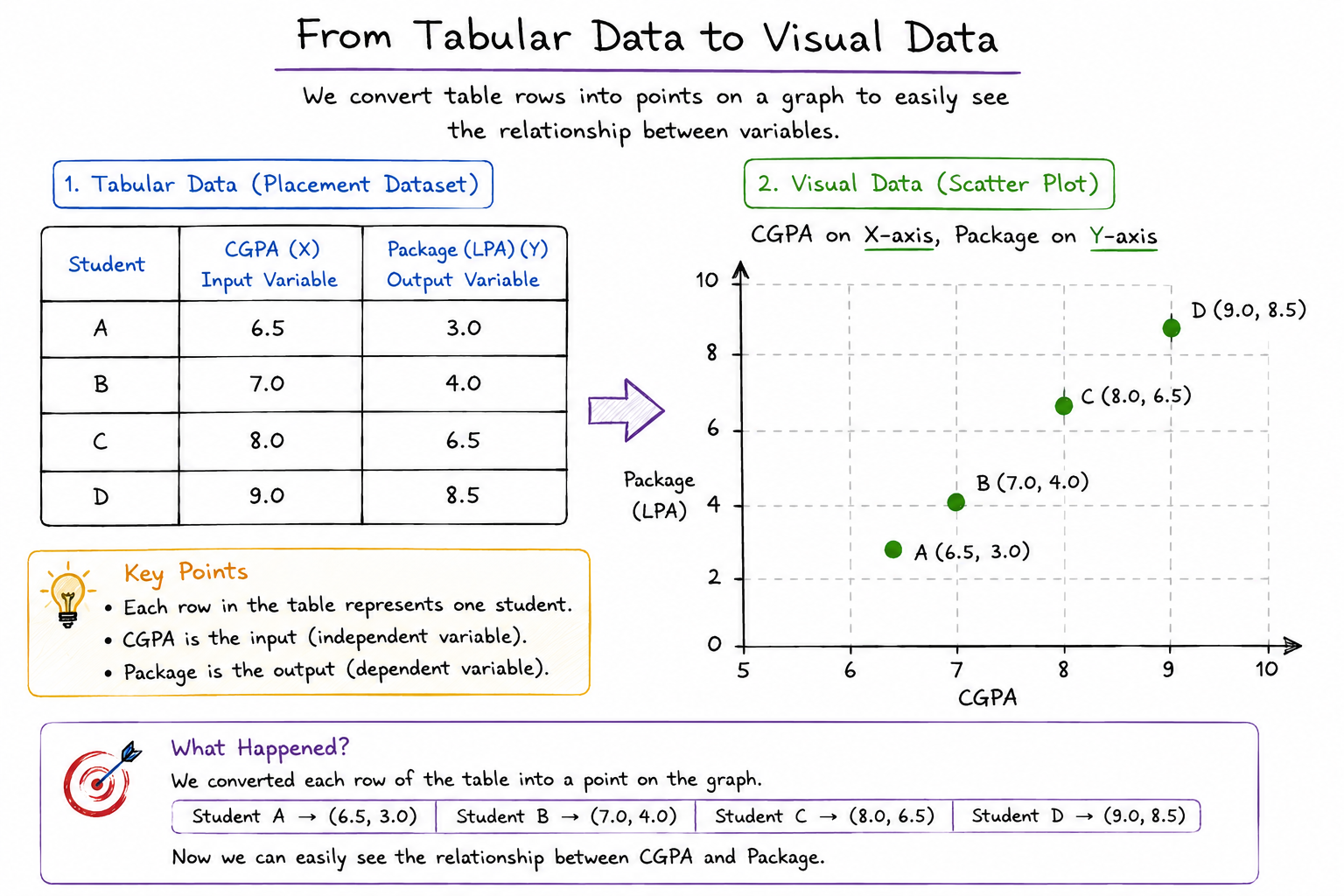
From Tabular Data to Visual Data
Earlier in this tutorial, we worked with a placement dataset where each row contained a student's CGPA and corresponding placement package.
| Student | CGPA | Package (LPA) |
|---|---|---|
| A | 6.5 | 3.0 |
| B | 7.0 | 4.0 |
| C | 8.0 | 6.5 |
| D | 9.0 | 8.5 |
Looking at this table allows us to read the data, but it does not immediately reveal patterns. Human beings are naturally good at recognizing visual patterns, which is why one of the first things a data scientist does is convert tabular data into a graphical representation. Instead of viewing rows and columns, we can represent each student as a point on a graph. The horizontal axis (X-axis) represents CGPA, while the vertical axis (Y-axis) represents the placement package. Every student contributes one point to the graph.
For example:
- Student A becomes the point (6.5, 3.0)
- Student B becomes the point (7.0, 4.0)
- Student C becomes the point (8.0, 6.5)
- Student D becomes the point (9.0, 8.5)
When all points are plotted together, we obtain a scatter plot.
What Is a Scatter Plot?
A scatter plot is a graphical representation of data where each observation is displayed as a point. The purpose of a scatter plot is to help us understand whether a relationship exists between two variables.
In our placement example:
- CGPA is placed on the X-axis.
- Package is placed on the Y-axis.
Every student becomes a dot on the graph. If students with higher CGPAs generally receive higher packages, the points will tend to move upward as we move from left to right. This visual pattern immediately tells us that some relationship may exist between CGPA and package. A scatter plot is often the first visualization created before applying Linear Regression because it helps us determine whether the data contains a meaningful trend.
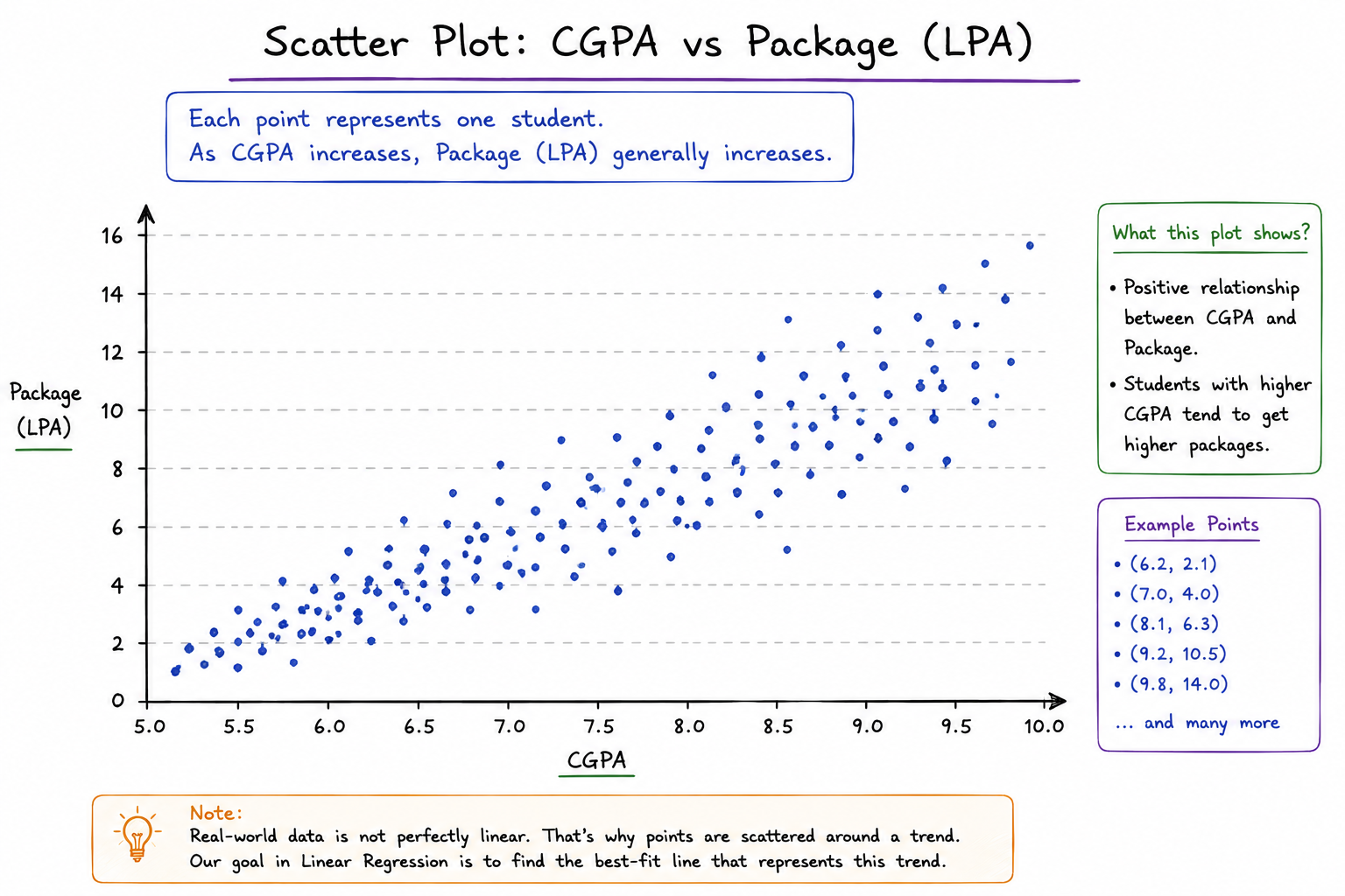
Understanding Correlation Through Visualization
Suppose we plot hundreds of students on the graph. As we observe the points, we may notice a general pattern.
Students with lower CGPAs often receive lower packages. Students with higher CGPAs often receive higher packages.
This suggests that both variables are moving in the same direction. When two variables tend to increase together, we say they have a positive relationship.
The graph may not be perfectly straight, but the overall trend becomes visible. This observation is extremely important because Linear Regression is based on the assumption that some underlying relationship exists between the input variable and the output variable. If no relationship exists at all, drawing a predictive line becomes meaningless.
Why Real-World Data Is Never Perfect
When beginners first learn Linear Regression, they often imagine that real-world data forms a perfectly straight line. In reality, almost no real-world dataset behaves that way.
Consider two students with the same CGPA. One student may perform exceptionally well in interviews. Another student may struggle during technical rounds. One student may have strong internship experience. Another student may have excellent communication skills. Some students may receive offers from high-paying multinational companies, while others may choose smaller organizations for personal reasons. Because of these factors, two students with similar CGPAs may receive very different packages.
As a result, the data points become scattered around the graph rather than lying exactly on a single line. This is completely normal.
In fact, if you encounter a real-world dataset where every point falls perfectly on a straight line, it is usually an indication that the dataset is artificial or highly simplified. Real-world data always contains variation, uncertainty, and noise.
Understanding Noise in Data
The differences that cannot be directly explained by our input variables are often called noise. Imagine that CGPA is the only feature available in our dataset.
However, package may also depend on:
- Communication skills
- Internship experience
- Project quality
- Interview performance
- Location preferences
- Company hiring policies
Since these factors are not included in the dataset, their influence appears as random variation. This variation causes points to spread around the graph. Noise is not a flaw in the dataset. Noise is simply a reflection of the complexity of the real world.
One of the goals of Machine Learning is to identify meaningful patterns despite the presence of noise.
What If the Data Were Perfectly Linear?
Before studying real-world scenarios, let us imagine an ideal situation. Suppose every student follows exactly the same relationship between CGPA and package.
The graph might look like this:
Package
 ^
 |
9|                *
8|             *
7|          *
6|       *
5|    *
4| *
 +--------------------> CGPA
Notice that every point lies perfectly on a straight line. In this case, finding the relationship is easy. We simply draw a line passing through all points.
Once the equation of that line is known, we can predict the package for any new student.
For example:
- CGPA = 7.5
- Substitute into the line equation
- Obtain the predicted package
Unfortunately, real-world datasets rarely behave this perfectly.
The Challenge with Real Data
Now consider a more realistic graph in which the points no longer fall exactly on a single line. Some points are above the trend. Some points are below the trend. Some points are farther away from where we might expect them to be.
At this stage, an important question arises:
How can we draw a single line that represents all these points?
This question leads directly to the concept of the best-fit line.
The Idea Behind the Best-Fit Line
Even though the points do not form a perfect line, they still appear to follow a general trend. The goal of Linear Regression is not to pass through every point. Instead, its goal is to find a line that represents the overall pattern in the data. This special line is called the Best-Fit Line.
The best-fit line acts as a summary of the entire dataset.
Instead of memorizing hundreds or thousands of observations, the model captures the overall relationship using a single mathematical equation. The line becomes a compact representation of the trend hidden inside the data.
Imagine drawing several different lines through the same scatter plot. Some lines may be too high. Some lines may be too low. Some lines may completely ignore the majority of points.
Clearly, not every line represents the data equally well. The best-fit line is the line that stays as close as possible to the majority of data points. In other words, it is the line that makes the smallest overall prediction mistakes.
If we compare multiple candidate lines, the best-fit line is the one that minimizes total error across all observations.
This idea of minimizing error is the heart of Linear Regression.
Making Predictions Using the Best-Fit Line
Once the best-fit line has been identified, prediction becomes straightforward.
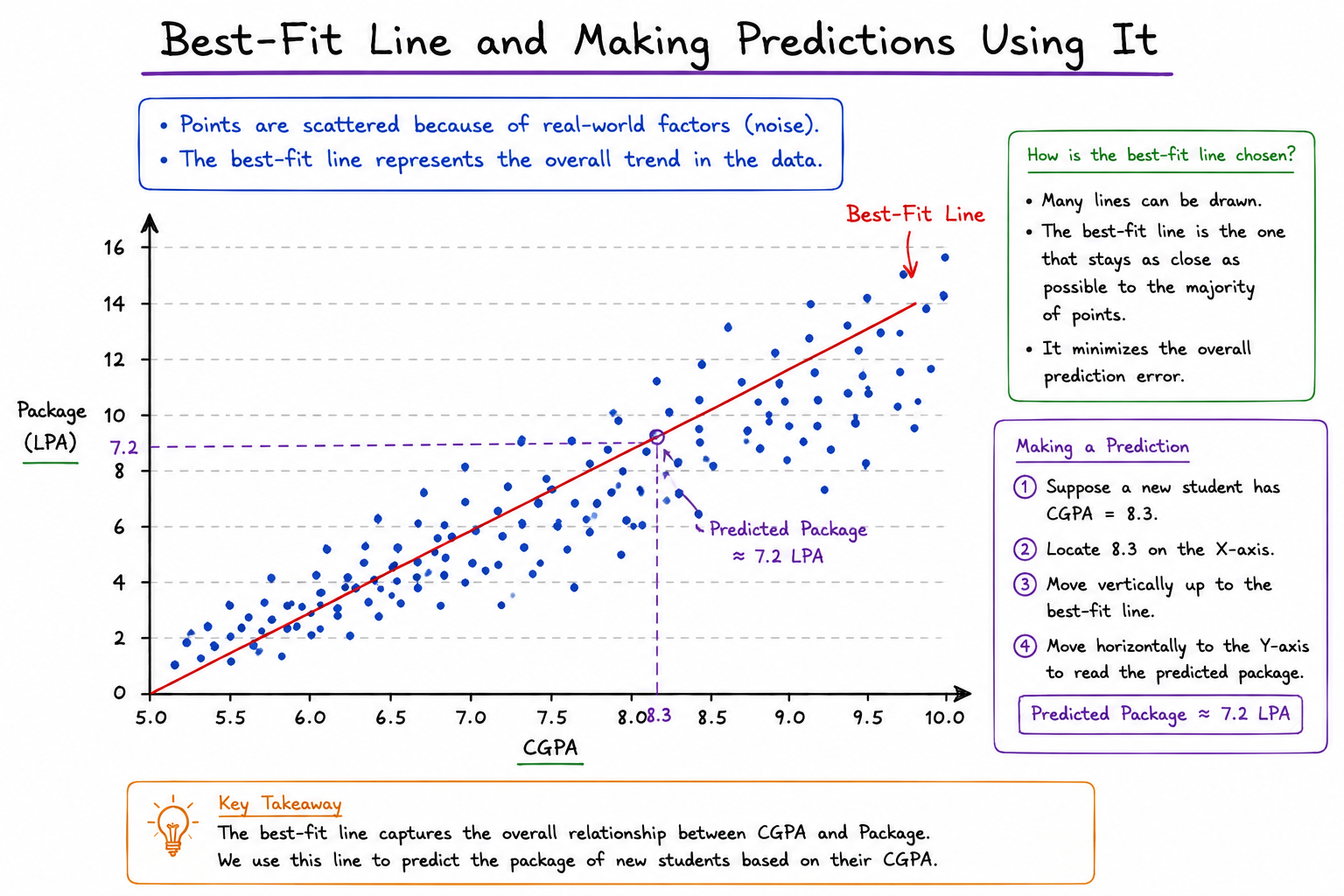
Suppose a new student arrives with a CGPA of 8.3. We locate 8.3 on the X-axis.
We move vertically until we reach the best-fit line. The corresponding Y-value becomes our predicted package.
The model is essentially answering the question:
"Based on the trend observed in historical data, what package would we expect for a student with this CGPA?"
The prediction may not be perfectly accurate because real-world outcomes contain uncertainty. However, the prediction is informed by historical evidence rather than guesswork.