Mathematical Representation of Simple Linear Regression

Introduction

In the previous sections, we learned that Linear Regression attempts to discover a best-fit line that captures the overall trend present in a dataset.

When we plotted student CGPAs against placement packages, we observed that the points were scattered around a general upward trend. Since the data was not perfectly linear, we introduced the concept of a best-fit line—a line that stays as close as possible to the majority of data points while minimizing overall prediction error. Visually, the idea is easy to understand. We can simply draw a line on the graph and use it to make predictions. However, a machine learning model cannot work with drawings.

A computer needs a mathematical representation of that line so that it can perform calculations automatically. Whenever a new student's CGPA is provided, the model should be able to compute the predicted package without drawing the graph again. This requirement leads us to one of the most important equations in Linear Regression.

The Equation of a Straight Line

If you have studied coordinate geometry, you may already be familiar with the equation of a straight line:

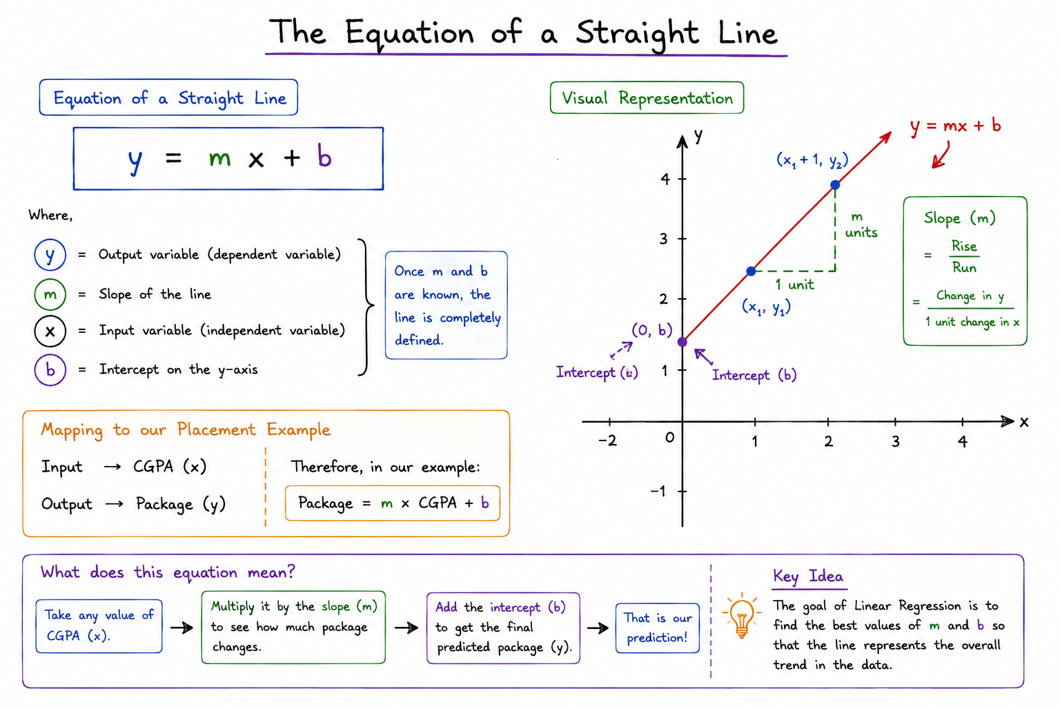
At first glance, this may appear to be an ordinary school-level mathematics formula. Surprisingly, this simple equation forms the foundation of the entire Linear Regression algorithm.

The equation describes a straight line using two parameters:

• A slope (m)
• An intercept (b)

Once these values are known, the line is completely defined. The goal of Linear Regression is to discover the most appropriate values of m and b so that the resulting line represents the trend hidden inside the dataset.

Mapping the Equation to Our Placement Prediction Problem

Mathematical symbols are easier to understand when they are connected to a real-world problem.

Throughout this tutorial, we have been working with a placement dataset where:

• CGPA is the input variable.
• Package is the output variable.

Therefore:

• x = CGPA
• y = Package

Substituting these values into the straight-line equation gives:

$$Package=m×CGPA+b$$

This equation tells us that the predicted package depends on two quantities learned from data:

• The slope (m)
• The intercept (b)

During training, the Linear Regression algorithm analyzes historical placement records and determines the best values of these parameters. Once those values have been found, predicting a package becomes a simple mathematical calculation.

Understanding the equation y = mx + b

Now, let us understand the equation.

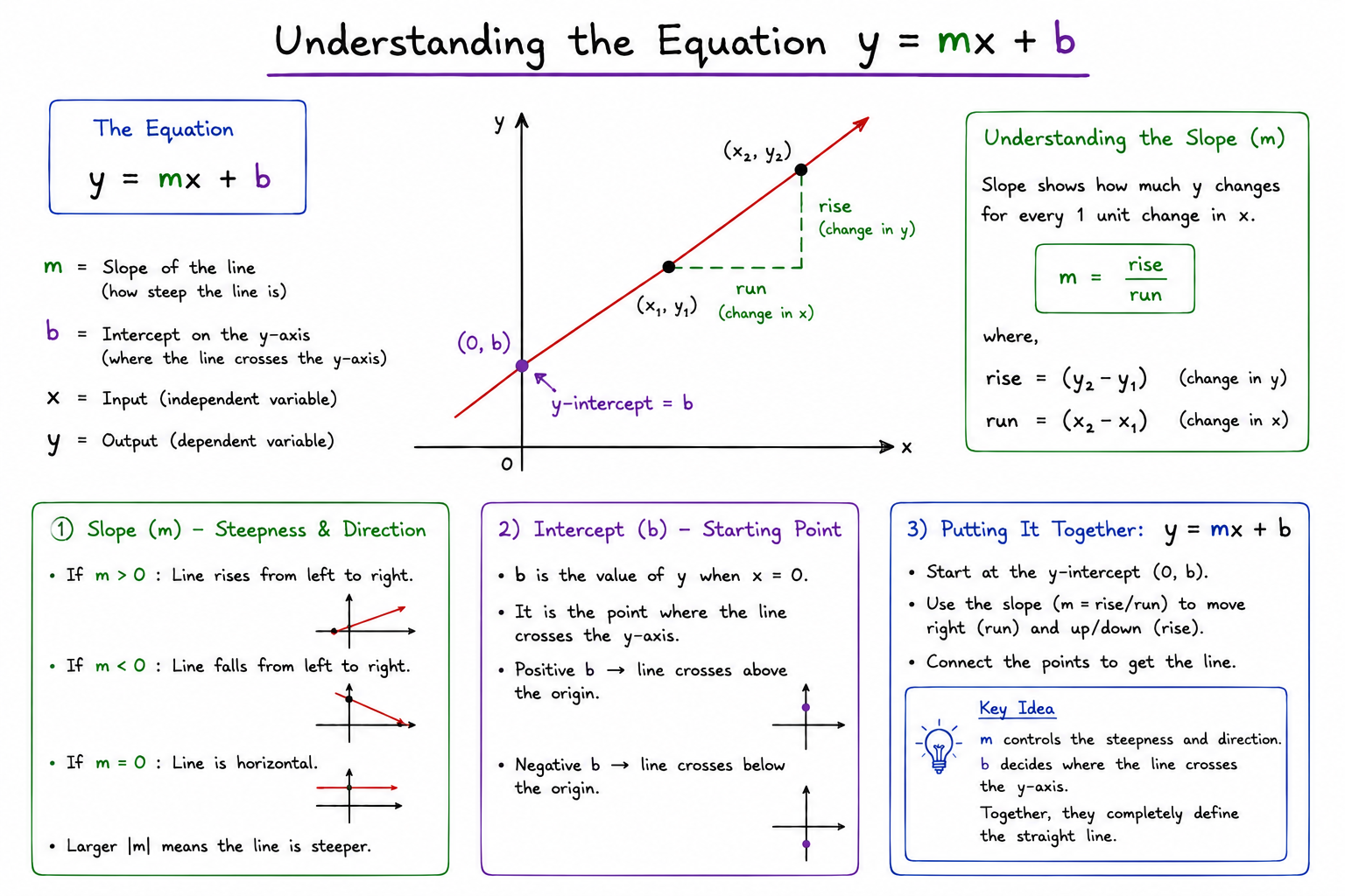
Understanding the Slope

The slope is one of the most intuitive concepts in Linear Regression. The slope tells us how much the output changes when the input increases by one unit.

In our placement example, the slope answers the following question:

"If a student's CGPA increases by one point, how much does the predicted package increase?"

This interpretation is extremely important because it allows us to understand how strongly CGPA influences the placement package.

Suppose the trained model learns the following equation:

$$Package=2×CGPA−10$$

Here: $m = 2$

This means that every one-point increase in CGPA increases the predicted package by approximately 2 LPA.

Consider the following predictions:

CGPA	Predicted Package
6	2 LPA
7	4 LPA
8	6 LPA
9	8 LPA

Notice what happens. Whenever CGPA increases by one unit, the package increases by two units. That increase is controlled entirely by the slope. In other words, the slope measures the rate at which the output variable changes as the input variable changes.

Visual Intuition Behind the Slope

Think back to the best-fit line. If the line rises very slowly, increasing CGPA will only slightly increase the predicted package. If the line rises very steeply, even a small increase in CGPA can produce a significant increase in the predicted package.

Therefore, the slope determines how steep the regression line appears on the graph.

• A larger slope produces a steeper line.
• A smaller slope produces a flatter line.

Because of this, the slope is often interpreted as the strength of the relationship between the input and output variables.

Many beginners find it easier to think about the slope as a measure of influence rather than as a mathematical quantity. For our placement problem, the slope answers:

"How much influence does CGPA have on package?"

• A larger slope means that CGPA plays a major role in determining the package.
• A smaller slope means that package is less sensitive to changes in CGPA.

This interpretation becomes particularly useful later when we study Multiple Linear Regression, where each feature receives its own coefficient representing its influence on the prediction.

Understanding the Intercept

The second parameter in the Linear Regression equation is the intercept.

While the slope determines how the line rises or falls, the intercept determines where the line begins. Mathematically, the intercept is the predicted value of the output when the input variable is zero.

To understand why, let us start with the regression equation:

Now suppose:

$$x=0$$

Substituting zero into the equation gives:

$$y=b$$

This means that the intercept represents the output value when the input variable is zero.

Interpreting the Intercept in Our Example

Suppose the model learns:

$$Package=2×CGPA+1$$

Here:

b = 1

According to the model, a student with a CGPA of zero would have a predicted package of 1 LPA. Now, this prediction may not be realistic because students with a CGPA of zero generally do not appear in placement datasets.

However, the intercept still serves an important purpose.

Its primary role is to position the regression line correctly on the graph. Without the intercept, the entire line might be shifted too high or too low, leading to poor predictions. For this reason, the intercept is often referred to as the baseline value of the prediction.

The slope and intercept define the entire regression line.

The intercept determines where the line starts. The slope determines how the line moves after that starting point. Together they create the mathematical model that Linear Regression uses for prediction.

A useful way to think about the equation is:

Prediction = (Input × Influence) + Baseline Value

Or, in our placement example:

Package = (CGPA × Slope) + Intercept

This interpretation is often easier to understand than memorizing mathematical symbols.