Why The Perceptron Learning Rule Is Not Enough

Introduction

In the previous tutorial, we learned about the Perceptron, one of the earliest and most influential machine learning models. We saw how a Perceptron takes input features, multiplies them by weights, adds a bias, and then applies an activation function to make a prediction.

We also learned a simple training strategy known as the Perceptron Learning Rule. The idea behind this rule is straightforward: whenever the Perceptron makes a mistake, we slightly adjust its weights and bias so that it becomes less likely to make the same mistake again. Repeating this process many times gradually moves the decision boundary toward a position that separates the classes.

At first glance, this approach seems sufficient. We start with random weights, keep updating them whenever mistakes occur, and eventually obtain a line that separates the data. This raises an important question:

If the Perceptron Learning Rule can already find a separating line, why do we need anything else?

The answer is that although the Perceptron Learning Rule works surprisingly well, it has several important limitations. Understanding these limitations will help us appreciate why concepts such as Loss Functions, Optimization, and Gradient Descent became fundamental parts of modern machine learning.

In this tutorial, we will examine the weaknesses of the Perceptron Learning Rule and understand why machine learning eventually moved toward loss-based optimization techniques.

Revisiting the Perceptron

Before discussing the limitations, let us briefly review what a Perceptron does.

Suppose we want to predict whether a student will get placed based on two features:

• CGPA
• IQ Score

The Perceptron receives these values as inputs.

$$x_1 = CGPA \\ x_2 =IQ$$

The weighted sum is calculated as:

$$z=w_1x_1 + w_2x_2+b$$

where:

• $w_1$ is the weight associated with CGPA
• $w_2$ is the weight associated with IQ
• b is the bias

The result is then passed through a Step Activation Function.

$$Output = \begin{array}{ll} 1 & \text{if } z \ge 0 \\ 0 & \text{if } z < 0 \end{array}$$

The output represents the predicted class.

Geometric Interpretation of a Perceptron

One of the most useful ways to understand a Perceptron is through geometry.

The equation

$$w_1x_1 + w_2x_2+b = 0$$

represents a straight line in a two-dimensional feature space. This line is known as the Decision Boundary.

The decision boundary divides the feature space into two regions:

• One region corresponds to class 0
• The other region corresponds to class 1

Every point on one side of the line belongs to one class, while every point on the other side belongs to the other class.

Because of this property, a Perceptron naturally performs binary classification.

For datasets with more dimensions, the line becomes a plane or, more generally, a hyperplane. However, the underlying idea remains exactly the same: the Perceptron tries to find a boundary that separates different classes.

Training a Perceptron

Prediction is only one part of machine learning. The more important task is training.

Training means finding suitable values of:

$$w_1, w_2, b$$

that correctly separate the classes. Earlier, we used the Perceptron Learning Rule for this purpose.

The process can be summarized as follows:

Step 1: Initialize Random Parameters

We begin with random values for weights and bias.

$$w_1 = random \\ w_2 = random \\ b = random$$

At this stage, the decision boundary is completely arbitrary.

Step 2: Select a Training Example

Pick a data point from the training dataset.

Step 3: Make a Prediction

Use the current decision boundary to predict the class of that point.

Step 4: Check for Mistakes

Compare the prediction with the actual label.

• If the prediction is correct, do nothing.
• If the prediction is incorrect, adjust the weights and bias.

Step 5: Repeat

Continue this process for many iterations until the decision boundary separates the classes.

This simple procedure is often referred to as the Perceptron Trick because it provides an intuitive way to train a Perceptron without requiring advanced mathematics.

Why the Perceptron Learning Rule Appears to Work

To understand the limitations, we must first understand why the rule works at all. Imagine that we have a decision boundary that incorrectly classifies some points.

Whenever a misclassified point is encountered, the Perceptron updates its weights. These updates effectively pull the decision boundary toward the misclassified point.

Over time:

• Incorrectly classified points influence the boundary.
• Correctly classified points do not influence the boundary.
• The boundary gradually moves into a better position.

Eventually, if the dataset is linearly separable, the Perceptron often finds a line that separates the two classes. This sounds excellent. However, there is a hidden problem.

The Fundamental Question

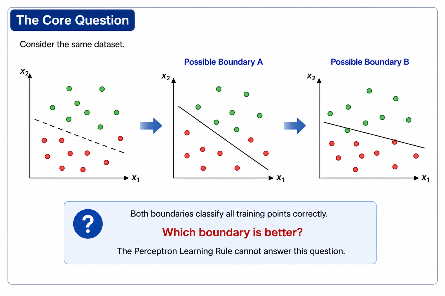
There are many possible ways to draw the line. Different lines can classify every point correctly.

Now ask yourself:

Which line is better?

The Perceptron Learning Rule cannot answer this question. This is where the real problem begins.

Problem 1: No Measure of Quality

Since all lines classify every training example correctly, the Perceptron Learning Rule treats them as equally good.

However, in reality, one boundary may be far more robust than the other. One boundary may leave a large margin between the classes, while another may pass dangerously close to some points.

The learning rule has no way of evaluating this difference. As a result, it cannot tell us whether we have found:

• A good solution
• A very good solution
• The best possible solution

It simply stops when classification becomes correct.

Problem 2: Different Runs May Produce Different Results

Another issue arises because the training process depends heavily on randomness.

Consider two independent training runs.

Run 1

• Random initialization
• Random sequence of training points
• Final boundary A

Run 2

• Different initialization
• Different sequence of training points
• Final boundary B

Both boundaries may classify the training data correctly. However, they may be completely different lines. Since the Perceptron Learning Rule does not provide a numerical measure of quality, there is no objective way to compare the two solutions. This means that running the same algorithm twice can lead to different outcomes, and we cannot confidently determine which outcome is superior.

Problem 3: All Mistakes Are Treated Equally

Imagine two misclassified points.

• Case 1: A point is only slightly on the wrong side of the decision boundary.
• Case 2: A point is very far from where it should be. Clearly, the second mistake is much more severe. However, the Perceptron Learning Rule treats both mistakes exactly the same.

The algorithm does not consider:

• How large the mistake is.
• How far the point is from the boundary.
• How confident the prediction was.

As a result, valuable information about prediction quality is ignored.

Problem 4: No Numerical Progress Indicator

When training a machine learning model, it is useful to monitor progress. The Perceptron Learning Rule does not naturally provide such a measure.

We can observe that the decision boundary is moving. We can observe that fewer mistakes are being made. However, we cannot quantify how much improvement has occurred.

There is no single number that continuously tells us:

"The model is becoming better."

Without such a measure, optimization becomes difficult.

Enter Loss Functions

A Loss Function is a mathematical function that measures how well or how poorly a model performs. Instead of merely declaring a prediction as correct or incorrect, a loss function assigns a numerical value representing the quality of the model.

For example:

$$Loss=100$$

might indicate a poor model.

After some training:

$$Loss=40$$

The model has improved.

After further training:

$$Loss=5$$

The model has improved even more. This simple idea provides several benefits:

• We can compare different models.
• We can compare different decision boundaries.
• We can monitor training progress.
• We can mathematically optimize model parameters.

Loss functions transformed machine learning from a collection of heuristics into a rigorous optimization problem.