Understanding The Perceptron Loss Function

Introduction

In the previous tutorial, we learned the Perceptron Trick. The Perceptron Trick gave us a practical way to train a Perceptron. Whenever a point was misclassified, we adjusted the decision boundary. After many such adjustments, the line gradually moved toward a position that separated the two classes.

The technique works surprisingly well, and for many simple datasets it is capable of finding a valid decision boundary. However, there is an important question that the Perceptron Trick does not answer.

How do we know whether the line we found is actually the best line? This question leads us to one of the most important concepts in machine learning Loss Functions. Before studying neural networks, backpropagation, or gradient descent, it is important to understand why loss functions exist and what problem they solve.

What We Really Need

Instead of simply asking "Is the classification correct", we would like to ask "How good is this line"?

Notice the difference.

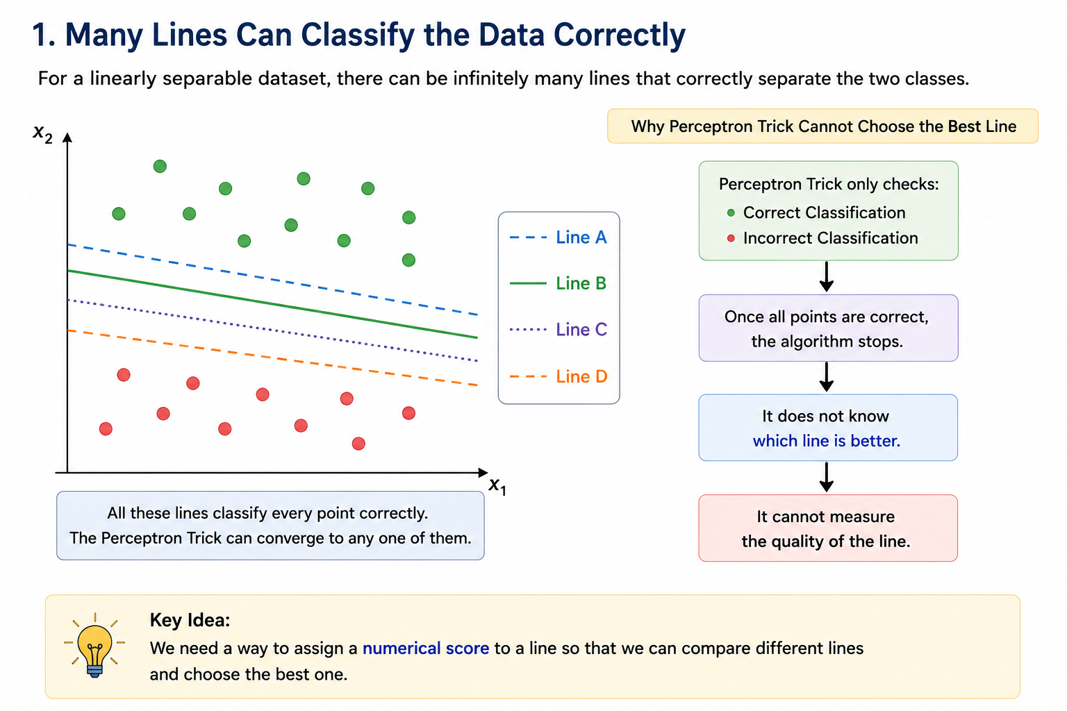
The first question produces only two answers:

• Yes
• No

The second question produces a numerical score.

For example:

• Line A → Score = 50
• Line B → Score = 20
• Line C → Score = 5

Now we can immediately conclude line C is the best line" because it has the smallest score. This numerical score is exactly what a loss function provides.

Thinking Like a Mathematician

Suppose someone gives you a line:

$$w_1x_1 + w_2x_2 + b = 0$$

and asks "How good is this line"?

One possible answer is: "Count the number of mistakes." This gives us our first candidate loss function.

First Attempt: Count Misclassified Points

Suppose a line misclassifies seven points. Then:

Loss = 7

Suppose another line misclassifies five points. Then:

Loss = 5

Clearly:

5 < 7

Therefore, the second line is better. At first glance, this seems like a perfectly reasonable loss function.

Why Counting Mistakes Is Not Enough

Consider these two situations.

Case 1

           ●

------------------

The point is just slightly on the wrong side.

Case 2

●





------------------

The point is far away from the decision boundary. Both situations count as 1 mistake. Yet intuitively they are not equally bad. In Case 1, the point needs only a tiny adjustment. In Case 2, the point requires a much larger correction. The simple counting approach cannot distinguish between these two situations. This is its biggest weakness.

A Better Idea: Measure Distance

Instead of counting mistakes, we can measure: "How far is a misclassified point from the decision boundary"?

Now consider the same two examples.

• Point Near the Boundary: Distance = 1
• Point Far From the Boundary: Distance = 10

Now the second mistake receives a larger penalty. This makes much more sense mathematically. Our loss can now be written as:

Loss =
Distance of Misclassified Point 1
+
Distance of Misclassified Point 2
+
...

This is already a much better loss function than simply counting errors.

The Problem With Distance Calculation

There is one issue. Calculating the perpendicular distance from every point to a line requires a more complicated formula.

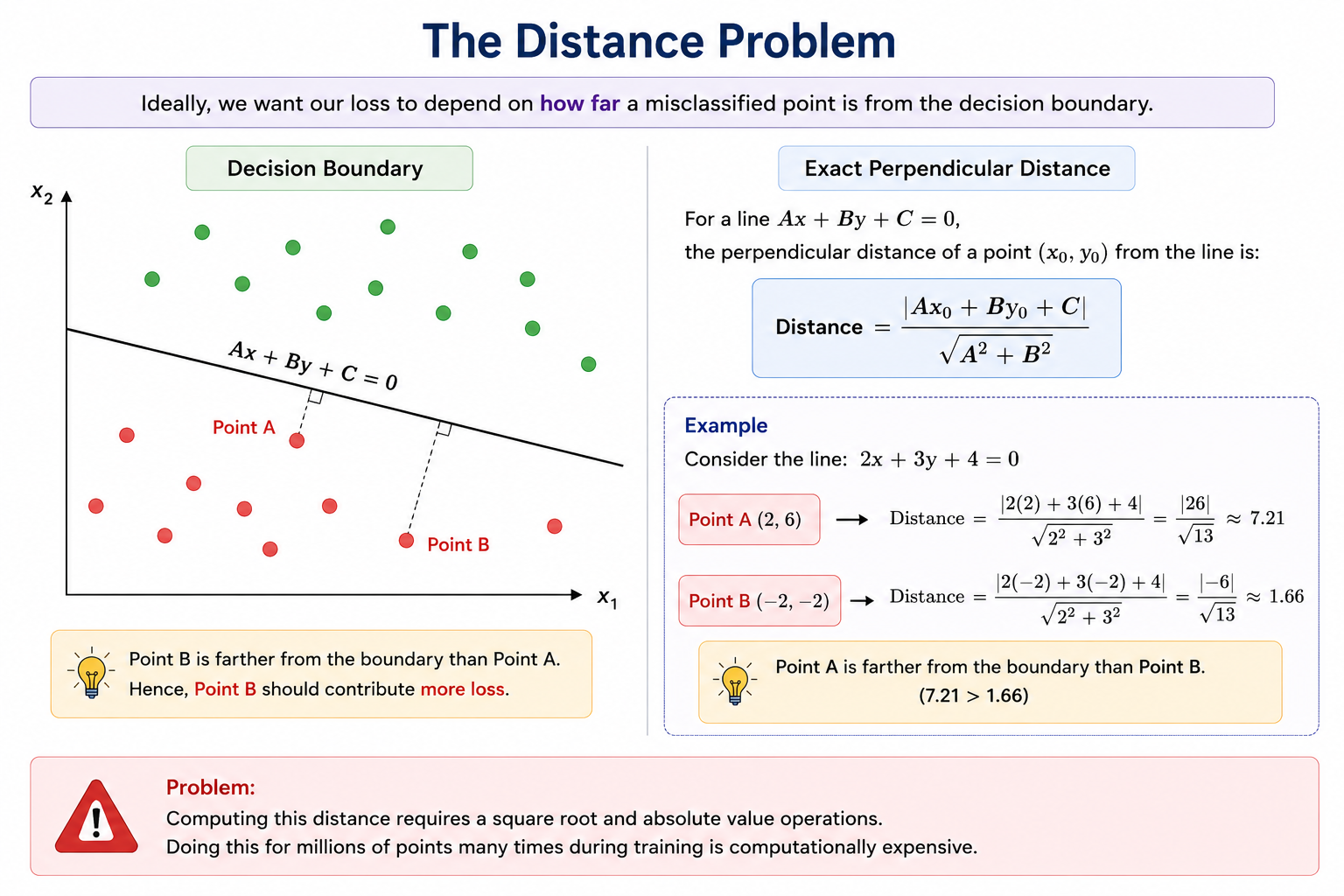
For a line:

$$Ax + By + C = 0$$

the distance of a point $(x_0,y_0)$ is

$\text{Distance} = \frac{|Ax_0 + By_0 + C|}{\sqrt{A^2 + B^2}}$ ​

This calculation is slightly expensive. Machine learning algorithms may need to perform it millions of times. Naturally, researchers looked for a simpler alternative.

An Interesting Observation

Suppose our line is:

$$2x+3y+4=0$$

Now take a point:

$$(2,6)$$

Substituting into the line equation:

$$2(2)+3(6)+4 =4+18+4 =26$$

Now consider another point:

$$(−2,−2)$$

Substituting:

$$2(−2)+3(−2)+4 =−4−6+4 =−6$$

Notice something interesting. Points farther from the boundary produce larger values. Points closer to the boundary produce smaller values. The exact distance is not being computed, but this quantity is strongly related to distance.

Therefore, instead of calculating the actual distance, we can use:

$$Ax+By+C$$

as a simpler measure of how badly a point is classified. This idea eventually leads to the mathematical form of the Perceptron Loss Function.

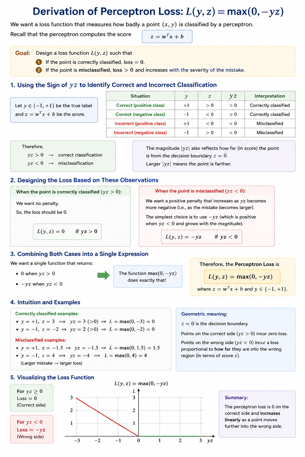
Mathematical derivation of loss function