Understanding Forward Propagation in a Multi-Layer Perceptron

Before we can understand how a neural network learns, we must first understand how it makes predictions.

When people begin studying neural networks, they often jump directly into Backpropagation because it is the algorithm responsible for training the network. However, Backpropagation only makes sense when you clearly understand what happens during the prediction phase. After all, before a neural network can learn from its mistakes, it must first produce an output. That output is generated through a process known as Forward Propagation.

This tutorial focuses entirely on that process. We will see how an input travels through multiple layers of a neural network, how weights and biases participate in the computation, and how Linear Algebra simplifies what would otherwise be a very complex set of calculations. The concepts discussed here are derived from the provided material.

Introduction: Why Forward Propagation Matters

A neural network is essentially a collection of interconnected neurons organized into layers. Each connection has an associated weight, and each neuron typically has a bias value.

When a new input enters the network, it does not immediately produce a prediction. Instead, the data passes through several layers where mathematical operations are performed repeatedly. The final result of these operations becomes the network's prediction.

This entire journey of data from the input layer to the output layer is called Forward Propagation.

In simple terms:

• Input enters the network.
• Mathematical transformations are performed layer by layer.
• The final output is produced.
• That output becomes the prediction of the model.

Only after this prediction is generated can the network compare it with the actual answer and begin learning through Backpropagation. Therefore, Forward Propagation is not just a preliminary topic; it is the foundation upon which the entire learning process is built.

** Forward Propagation vs Backpropagation

To understand the role of Forward Propagation in a neural network, it is helpful to compare it with Backpropagation. These two processes work together during training, but they serve very different purposes.

Forward Propagation is the process through which information flows from the input layer toward the output layer. The network receives the input features, performs a series of mathematical computations at each neuron, and gradually transforms the input into a final prediction. During this stage, the network is simply using its current weights and biases to produce an output. No learning or parameter updates occur. The objective of Forward Propagation is only to answer the question: "Given the current state of the network, what prediction does it make?"

Once a prediction has been generated, the network compares that prediction with the actual target value and calculates the error. This is where Backpropagation begins. Instead of moving information from left to right, Backpropagation sends error information in the opposite direction, from the output layer back toward the input layer. As the error travels backward through the network, it determines how much each weight and bias contributed to the mistake. Using this information, the optimization algorithm updates the network parameters so that future predictions become more accurate.

In simple terms, Forward Propagation is responsible for making predictions, while Backpropagation is responsible for learning from mistakes. Forward Propagation tells us what the network currently believes, whereas Backpropagation tells us how the network should adjust itself to improve those beliefs.

A useful way to think about the relationship between the two is that Forward Propagation answers the question:

"What prediction does the network make?"

while Backpropagation answers the question:

"How should the network change its weights and biases so that future predictions become better?"

Because the learning process cannot begin until a prediction has first been produced, Forward Propagation always occurs before Backpropagation. For this reason, understanding Forward Propagation is an essential first step before studying how neural networks learn and update their parameters.

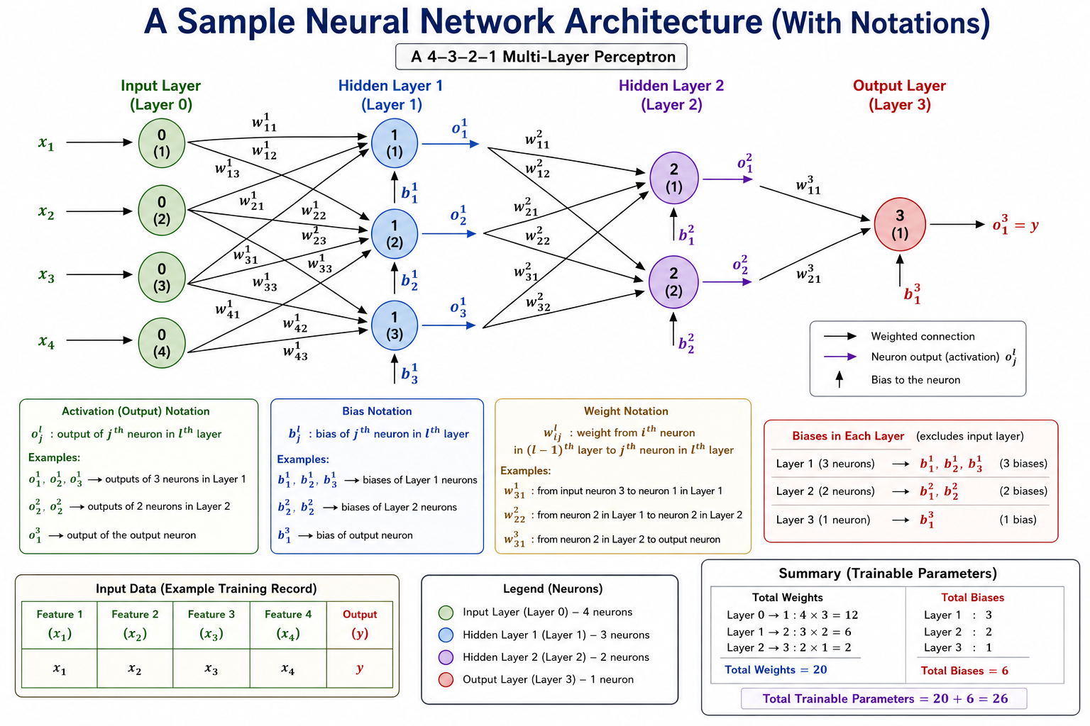
A Sample Neural Network Architecture

Consider a neural network with:

• 4 input neurons
• First hidden layer containing 3 neurons
• Second hidden layer containing 2 neurons
• 1 output neuron

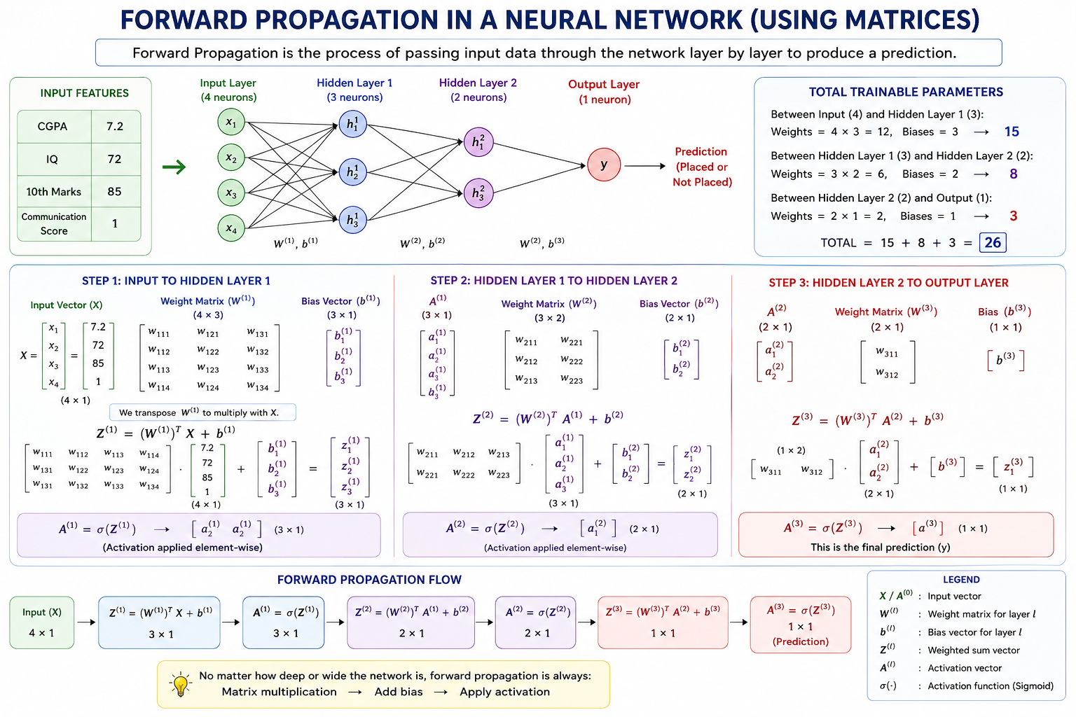
Visually, the architecture looks like this:

Representing Inputs as a Vector

Our input row can be represented as:

$$X = \begin{bmatrix} 7.2 \\ 72 \\ 85 \\ 1 \end{bmatrix}$$

This is a column vector containing all input features. Instead of treating features separately, we now treat them as a single mathematical object.

Creating the Weight Matrix

For the first hidden layer we have:

• 4 inputs
• 3 neurons

The weight matrix contains all connections between these layers.

$$W^{(1)}$$

contains 12 weight values.

Similarly,

$$B^{(1)}$$

contains the bias values of Hidden Layer 1.

Computing the First Hidden Layer

The entire first hidden layer can be computed using a single matrix equation:

$$Z^{(1)}=(W^{(1)})^TX+B^{(1)}$$

This produces a vector containing the weighted sums for all neurons in Hidden Layer 1.

Next, the activation function is applied:

A^1=σ(Z^1)

The result becomes the input to the next layer. Notice how we did not calculate each neuron individually. One matrix multiplication handled the entire layer.

This is one of the biggest reasons why Linear Algebra is central to Deep Learning.

Moving Through the Network Layer by Layer

The same process repeats for every layer.

For Hidden Layer 2:

$$Z^{(2)}=(W^{(2)})^TA^{(1)}+B^{(2)}$$

Apply activation:

$$A^{(2)}=σ(Z^{(2)})$$

For the Output Layer:

$$Z^{(3)}=(W^{(3)})^TA^{(2)}+B^{(3)}$$

Apply activation:

$$A^{(3)}=σ(Z^{(3)})$$

The value $A^{(3)}$ becomes the final prediction.

What Actually Happens During Prediction?

Let us summarize the prediction process.

When a new input record arrives:

1. Input values enter the network.
2. Matrix multiplication is performed using weights.
3. Biases are added.
4. Activation functions are applied.
5. Outputs become inputs for the next layer.
6. The process repeats until the final layer.
7. The final activation becomes the prediction.

That is all Forward Propagation really is. Although the architecture may appear complex, every layer performs the same sequence of operations repeatedly.

Forward Propagation Through the Lens of Linear Algebra

This section should come after introducing the neural network architecture and before introducing the generalized forward propagation equations.

Why Do We Need Matrices?

When people first learn neural networks, they usually calculate the output of each neuron individually.

For example, if a neuron receives four inputs, its output can be calculated as:

$$z=w_1​x_1​+w_2​x_2​+w_3​x_3​+w_4​x_4​+b$$

This approach works well when there is only one neuron. However, a real neural network contains many neurons in every layer. If we continue calculating every neuron separately, the amount of mathematical work quickly becomes overwhelming.

Imagine a network with:

• 100 input features
• 50 neurons in the first hidden layer
• 20 neurons in the second hidden layer

Computing every neuron individually would be tedious and inefficient.

Fortunately, Linear Algebra provides a much cleaner solution. Instead of treating neurons one at a time, we group inputs, weights, biases, and outputs into vectors and matrices. Once this is done, an entire layer can be computed using a single matrix multiplication operation.

This is the reason modern deep learning libraries such as TensorFlow and PyTorch rely heavily on matrix operations.

Step 1: Represent the Input as a Vector

Suppose we are predicting whether a student will get placed based on four features:

Feature	Value
CGPA	7.2
IQ	72
10th Marks	85
Communication Score	1

Instead of treating these values separately, we combine them into a column vector:

$$A^{(0)} = X = \begin{bmatrix} 7.2 \\ 72 \\ 85 \\ 1 \end{bmatrix}$$

Notice the notation $A^{(0)}$. The superscript 0 indicates that this is the activation of Layer 0, which is simply the input layer.

The dimensions of this vector are:

$$4×1$$

because it contains four rows and one column.

Step 2: Organize the Weights into a Matrix

The first hidden layer contains three neurons.

Since every input neuron connects to every neuron in Hidden Layer 1, we have:

$$4×3=12$$

weights.

Using proper mathematical notation, the weight matrix becomes:

$$W^{(1)} = \begin{bmatrix} w_{11}^{(1)} & w_{12}^{(1)} & w_{13}^{(1)} \\ w_{21}^{(1)} & w_{22}^{(1)} & w_{23}^{(1)} \\ w_{31}^{(1)} & w_{32}^{(1)} & w_{33}^{(1)} \\ w_{41}^{(1)} & w_{42}^{(1)} & w_{43}^{(1)} \end{bmatrix}$$

This matrix has dimensions:

$$4×3$$

Each column represents all the weights feeding into one hidden neuron.

Step 3: Why Do We Transpose the Weight Matrix?

Our input vector has dimensions:

$$4×1$$

while the weight matrix has dimensions:

$$4×3$$

Matrix multiplication requires the inner dimensions to match.

Therefore:

$$(4×3)×(4×1)$$

is invalid. To solve this problem, we transpose the weight matrix:

$$(W^{(1)})^T$$

After transposition:

$$(W^{(1)})^T=3×4$$

Now multiplication becomes possible:

$$(3×4)×(4×1)=(3×1)$$

The resulting vector contains one value for each neuron in the hidden layer.

Step 4: Computing the Weighted Sum

The weighted input to Hidden Layer 1 is:

$$Z^{(1)}=(W^{(1)})^TA^{(0)}+B^{(1)}$$

where

$$B^{(1)} = \begin{bmatrix} b_{1}^{(1)} \\ b_{2}^{(1)} \\ b_{3}^{(1)} \end{bmatrix}$$

is the bias vector.

The dimensions are:

$$(3×4)×(4×1)+(3×1)=(3×1)$$

The result looks like:

$$Z^{(1)} = \begin{bmatrix} z_{1}^{(1)} \\ z_{2}^{(1)} \\ z_{3}^{(1)} \end{bmatrix}$$

Each value represents the weighted sum for one neuron.

What Is Actually Happening Behind the Matrix Multiplication?

Although matrix multiplication looks complicated, it is simply performing multiple dot products simultaneously.

For example, the first neuron computes:

$$z_{1}^{(1)} = w_{11}^{(1)}x_1 + w_{21}^{(1)}x_2 + w_{31}^{(1)}x_3 + w_{41}^{(1)}x_4 + b_{1}^{(1)}$$

The second neuron computes:

$$z_{2}^{(1)} = w_{12}^{(1)}x_1 + w_{22}^{(1)}x_2 + w_{32}^{(1)}x_3 + w_{42}^{(1)}x_4 + b_{2}^{(1)}$$

The third neuron performs a similar calculation. The matrix multiplication simply performs all three computations at once. This is the real power of Linear Algebra.

Step 5: Applying the Activation Function

The weighted sums are then passed through an activation function.

Using the sigmoid function:

$$A^{(1)}=σ(Z^{(1)})$$

Result:

$$A^{(1)} = \begin{bmatrix} a_{1}^{(1)} \\ a_{2}^{(1)} \\ a_{3}^{(1)} \end{bmatrix}$$

This vector now becomes the input to the next layer.

Repeating the Same Process for the Next Layer

The second hidden layer contains two neurons.

Therefore:

$$W^{(2)}=3×2$$

After transposition:

$$(W^{(2)})^T=2×3$$

Forward propagation for the second hidden layer becomes:

$$Z^{(2)}=(W^{(2)})^TA^{(1)}+B^{(2)}$$

followed by:

$$A^{(2)}=σ(Z^{(2)})$$

The dimensions now become:

$$(2×3)×(3×1)=(2×1)$$

The network has compressed three activation values into two.

Computing the Final Prediction

The output layer contains a single neuron.

Therefore:

$$W^{(3)}=2×1$$

and:

$$(W^{(3)})^T=1×2$$

The final computation becomes:

$$Z^{(3)}=(W^{(3)})^TA^{(2)}+B^{(3)}$$

followed by:

$$A^{(3)}=σ(Z^{(3)})$$

Since the result has dimensions:

$$1×1$$

it is a single number. That number is the final prediction produced by the neural network.