Training a Perceptron: Understanding the Perceptron Trick

Introduction

In the previous discussion about the Perceptron, we learned that it is one of the simplest forms of an artificial neural network capable of performing binary classification. Given a set of input features, a perceptron calculates a weighted sum, compares it against a threshold, and predicts one of two possible classes.

However, a very important question still remains unanswered:

How does a perceptron determine the correct values of its weights and bias?

This is one of the fundamental questions in machine learning. Initially, a perceptron starts with random values for its weights and bias. These random values rarely produce accurate predictions, which means the model must gradually improve them by learning from the training data.

The process through which a perceptron learns these values is known as the Perceptron Learning Algorithm, and the intuition behind this learning process is often explained using what is commonly called the Perceptron Trick.

In this tutorial, we will build a strong geometric understanding of how a perceptron learns, how it modifies its decision boundary, and how repeated corrections eventually lead to a well-trained classification model.

Recap: What Does a Perceptron Actually Learn?

Before discussing how a perceptron is trained, it is important to first understand what the perceptron is actually trying to learn from the data.

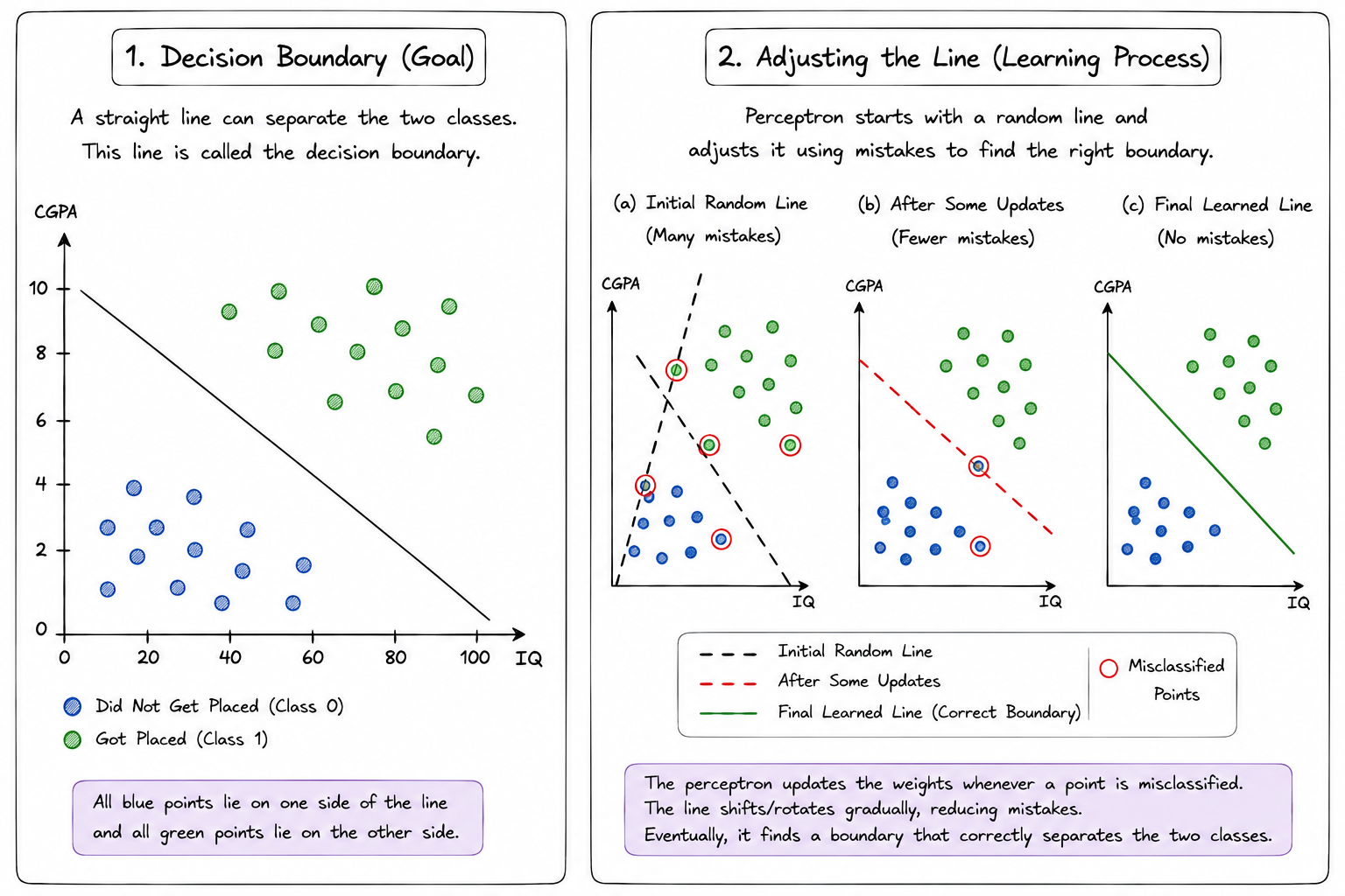
Consider a dataset containing two classes of points. For example, imagine a dataset of students where one class represents students who got placed and the other class represents students who did not get placed. If we plot these students on a graph using features such as IQ and CGPA, we may observe that the two groups occupy different regions of the graph.

If it is possible to draw a single straight line that separates these two groups, then the dataset is said to be linearly separable. In such a scenario, all points belonging to one class lie on one side of the line, while points belonging to the other class lie on the opposite side.

The primary objective of the perceptron is to discover this separating line, which is known as the decision boundary. Once the correct decision boundary has been found, the perceptron can classify new data points simply by determining on which side of the boundary they fall.

Initially, however, the perceptron has no knowledge of where this decision boundary should be located. It starts with randomly initialized weights and bias, which correspond to a randomly positioned line. As the training process progresses, the perceptron continuously adjusts this line based on its mistakes, gradually moving it closer to the ideal position. Therefore, training a perceptron can be viewed as the process of repeatedly modifying a decision boundary until it becomes an effective separator between different classes.

Understanding Linearly Separable Data

Let us imagine a dataset containing blue points and green points.

Visually, if you can draw a straight line such that:

• All blue points lie on one side.
• All green points lie on the other side.

then the dataset is linearly separable.

The line shown above acts as a boundary between the two classes. In two dimensions, this boundary is called a decision boundary.

In higher dimensions, it becomes a hyperplane, but the underlying concept remains exactly the same. The entire goal of perceptron training is therefore: Find the correct decision boundary that separates the classes.

The Decision Boundary Equation

A perceptron represents its decision boundary using a linear equation.

For two input features, the equation is:

$w_1x_1+w_2x_2+b=0$

where:

• $x_1$ and $x_2$ are input features.
• $w_1$ and $w_2$ are weights.
• $b$ is the bias.

This equation represents a straight line.

Every point located on one side of the line belongs to one class, while points on the other side belong to another class. The challenge is that the perceptron initially does not know the correct values of these parameters. Therefore, the first line is usually a poor separator. Training gradually improves these parameters until the line reaches a better position.

The Core Idea Behind the Perceptron Trick

Suppose the perceptron starts with a random line. Unfortunately, this line may classify many points incorrectly. Some blue points may appear inside the green region, and some green points may appear inside the blue region.

The perceptron follows a surprisingly simple strategy:

• Select a training point.
• Check whether it is classified correctly.
• If it is classified correctly, do nothing.
• If it is classified incorrectly, adjust the line slightly.
• Repeat this process many times.

Rather than searching directly for the perfect decision boundary, the perceptron continuously improves itself by correcting mistakes. Each correction slightly changes the position or orientation of the line. After many such corrections, the line gradually approaches a configuration that separates the classes correctly. This learning strategy is known as the Perceptron Trick.

Understanding Positive and Negative Regions

To understand how predictions are made, we must first understand the concepts of positive and negative regions.

Consider the line:

$$2x+3y+5=0$$

Suppose we take any point $(x,y)$ and substitute it into the equation.

Case 1: Result is Positive

$$2x+3y+5>0$$

The point lies in the positive region.

Case 2: Result is Negative

$$2x+3y+5<0$$

The point lies in the negative region.

By simply checking whether the equation produces a positive or negative value, we can determine on which side of the line a point lies. This simple observation forms the foundation of perceptron prediction.

How a Perceptron Makes Predictions

For every input point, the perceptron calculates:

$$z=w_1x_1+w_2x_2+b$$

The sign of $z$ determines the prediction.

If:

$$z≥0$$

the perceptron predicts Class 1.

If:

$$z<0$$

the perceptron predicts Class 0. Notice what is happening here.

The perceptron is essentially checking which side of the decision boundary contains the point. A positive value indicates that the point lies in the positive region, while a negative value indicates that it lies in the negative region.

This simple sign check allows the perceptron to perform classification.

Understanding Line Transformations

To understand how learning works, we must understand how changing the coefficients affects the line.

Consider the general equation:

$$ax+by+c=0$$

Changing different coefficients causes different transformations.

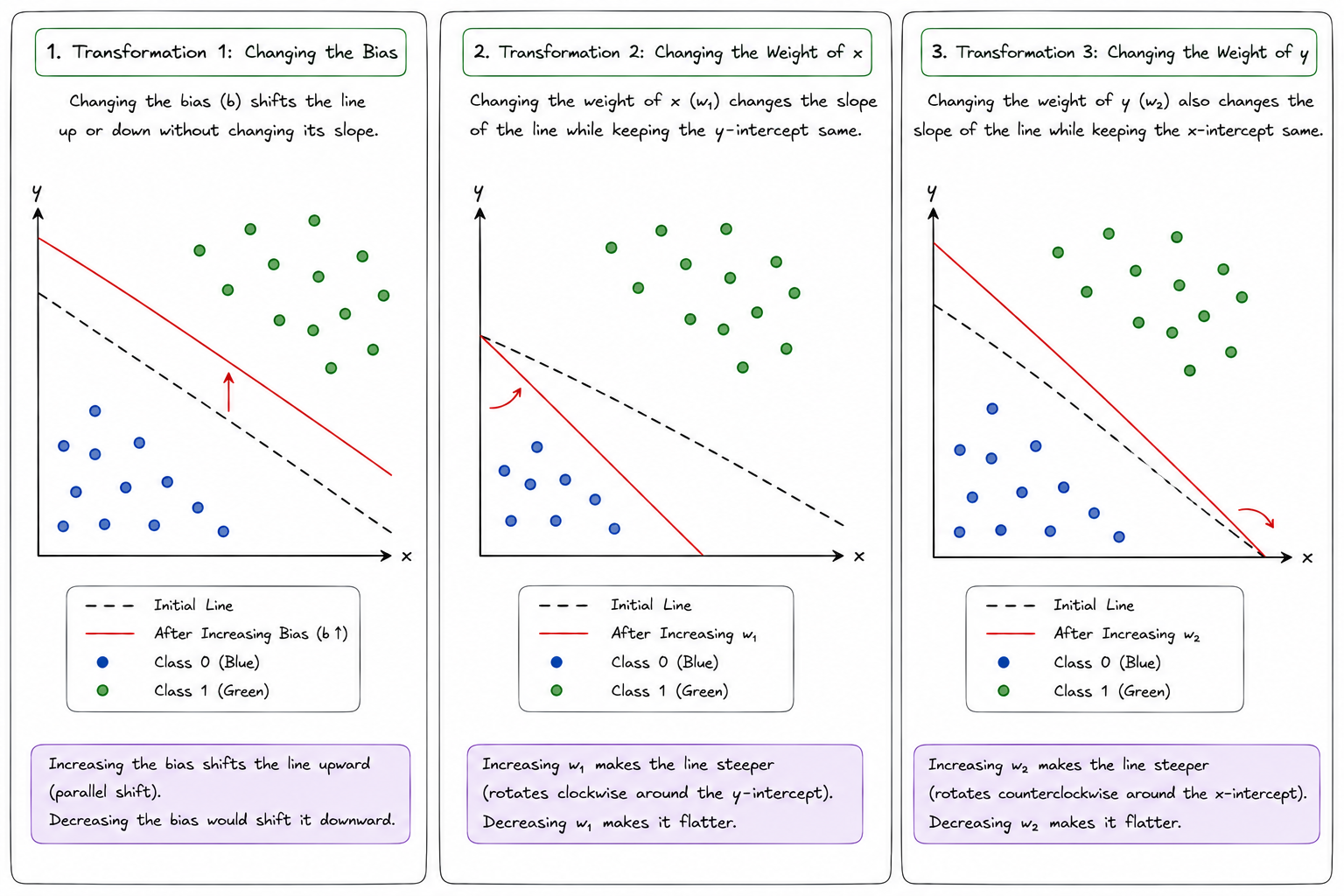
Transformation 1: Changing the Bias

Suppose we start with:

$$2x+3y+5=0$$

and change it to:

$$2x+3y+10=0$$

The slope remains unchanged. Only the position of the line changes. The line moves parallel to itself. This movement is called translation. Therefore, changing the bias shifts the line upward or downward without changing its orientation.

Transformation 2: Changing the Weight of x

Suppose we modify the coefficient of $x$.

$$2x+3y+5=0$$

becomes

$$5x+3y+5=0$$

Now the slope changes. The line rotates.

Therefore, modifying $w_1$ causes the decision boundary to rotate.

Transformation 3: Changing the Weight of y

Suppose we modify the coefficient of $x$.

$$2x+3y+5=0$$

becomes

$$5x+3y+5=0$$

Again, the orientation changes. The line rotates differently.Therefore, changing $w_2$ also affects the slope of the decision boundary.

Why Misclassified Points Are Important

Suppose a blue point accidentally falls inside the green region. This means the current decision boundary is incorrect.

The point is effectively telling the model:

"The boundary is not positioned correctly. Move it closer to me."

Misclassified points contain valuable information because they reveal where the model is making mistakes. Correctly classified points do not require any action.

The perceptron therefore focuses only on examples that are classified incorrectly. Every weight update is triggered by a mistake. This idea is extremely important because it forms the basis of the entire learning algorithm.

Representing the Bias as an Additional Weight

To simplify calculations, we usually represent the bias as an additional weight.

Instead of writing:

$$w_1​x_1​+w_2​x_2​+b$$

we write:

$$w_0​x_0​+w_1​x_1​+w_2​x_2​$$

where:

$$x_0​=1$$

This allows us to treat the bias exactly like any other weight.

The input vector becomes:

$$X=[1,x_1​,x_2​]$$

and the weight vector becomes:

$$W=[w_0​,w_1​,w_2​]$$

This representation greatly simplifies the training algorithm.

The Perceptron Weight Update Rule

Suppose a point belongs to the negative class but is incorrectly classified as positive. The perceptron must move the decision boundary away from that point.

The update rule becomes:

$$W_{new}=W_{old}-\eta X$$

where:

• $W$ is the weight vector.
• $X$ is the input vector.
• $η$ is the learning rate.

Now consider the opposite situation. A positive point has been incorrectly classified as negative. The perceptron must move the decision boundary toward that point.

The update rule becomes:

$$W_{new}=W_{old}+\eta X$$

These simple updates gradually shift and rotate the decision boundary in the correct direction.

Why Do We Need a Learning Rate?

Imagine applying huge corrections every time a mistake occurs. The decision boundary would jump wildly across the graph. Learning would become unstable.

To prevent this, we introduce a small constant known as the learning rate.

The learning rate is represented by $η$ (pronounced as eta).

Common values include:

$$0.1,0.01,0.001$$

Instead of making large corrections, the perceptron makes small, controlled adjustments. This allows the model to learn gradually and more reliably.

The Complete Perceptron Training Algorithm

Now that we understand decision boundaries, positive and negative regions, weight updates, and the role of the learning rate, we can combine all these concepts into a complete training procedure. The goal of the algorithm is to repeatedly identify mistakes made by the perceptron and use those mistakes to gradually improve the position of the decision boundary.

At a high level, the perceptron follows a very simple learning strategy. It starts with random weights, makes predictions on training examples, checks whether those predictions are correct, and updates the weights whenever it encounters a misclassified point. Over time, these updates cause the decision boundary to shift and rotate until it separates the classes more effectively.

Step 1: Initialize the Weights

The training process begins by assigning random values to all weights and the bias.

$$W=[w_0​,w_1​,w_2​]$$

Since the weights are chosen randomly, the initial decision boundary is also random and is unlikely to classify the training data correctly.

Step 2: Repeat the Training Process for Multiple Epochs

The perceptron does not learn from a single example. Instead, it repeatedly processes the training data. An epoch represents one complete cycle of training. During each epoch, the perceptron examines training examples, evaluates its predictions, and updates the weights whenever necessary. The algorithm continues for a fixed number of epochs or until the model stops making mistakes.

Step 3: Select a Training Example

Next, choose a training example from the dataset. For a dataset containing IQ and CGPA values, a training point may look like:

$$X=[1,75,8.2]$$

The leading value 1 represents the bias input.

Each training example contains:

• Input features
• Actual class label

The actual label tells us whether the point belongs to Class 0 or Class 1.

Step 4: Calculate the Weighted Sum

The perceptron computes the weighted sum of all inputs.

$$z=w_0​+w_1​x_1​+w_2​x_2​$$

​ This value determines on which side of the decision boundary the point lies.

You can think of this step as asking:

"Based on my current decision boundary, should this point belong to the positive region or the negative region?"

Step 5: Generate a Prediction

The weighted sum is converted into a prediction using a simple threshold rule. If:

$$z≥0$$

the perceptron predicts:

$$\hat{y}=1$$

Otherwise:

$$\hat{y}=0$$

At this stage, the perceptron has made its guess, but it still does not know whether that guess is correct.

Step 6: Compare the Prediction with the Actual Label

Now the perceptron compares:

• Predicted label $\hat{y}$
• Actual label $y$

Two situations are possible.

Case 1: Correct Prediction

If:

$$\hat{y}=y$$

the perceptron has classified the point correctly. In this case, no update is required because the current decision boundary already handles this point correctly. The algorithm simply moves to the next training example.

Case 2: Incorrect Prediction

If:

$$\hat{y}\ne y$$

the point has been misclassified.

This indicates that the decision boundary is not positioned correctly and must be adjusted.

Step 7: Update the Weights

This is the most important step of the algorithm. The perceptron modifies its weights whenever it encounters a mistake.

Positive Point Classified as Negative

Suppose the actual label is:

$$y=1$$

but the perceptron predicts:

$$\hat{y}=0$$

This means a positive point has fallen into the negative region. To correct the mistake, the decision boundary must move toward that point.

The weight update rule becomes:

$$W_{new}​=W_{old}​+ηX$$

where:

• $η$ is the learning rate.
• $X$ is the input vector.

Negative Point Classified as Positive Suppose the actual label is:

$$y=0$$

but the perceptron predicts:

$$\hat{y}=1$$

This means a negative point has fallen into the positive region. The decision boundary must move away from that point. The update rule becomes:

$$W_{new}​=W_{old}​−ηX$$

Each update causes a small shift or rotation of the decision boundary, gradually reducing the number of classification errors.

Step 8: Continue Until Convergence

The perceptron repeats the same process again and again:

1. Select a training example.
2. Make a prediction.
3. Check for errors.
4. Update the weights if necessary.

Over time, the number of mistakes decreases. For linearly separable datasets, the decision boundary eventually reaches a position where all training examples are classified correctly. At that point, the perceptron is said to have converged, and the training process can stop.

Visualizing the Entire Process

The complete training cycle can be summarized as:

Initialize Weights
        ↓
Select Training Point
        ↓
Calculate Weighted Sum
        ↓
Make Prediction
        ↓
Prediction Correct?
      /      \
    Yes      No
     |        |
 No Update  Update Weights
     |        |
     └──> Next Example
                ↓
         Repeat Process
                ↓
           Convergence

Notice that the perceptron does not directly search for the perfect decision boundary. Instead, it learns through a series of small corrections. Every misclassified point provides information about how the boundary should move, and the repeated accumulation of these small adjustments eventually produces a decision boundary that separates the classes effectively. This simple mistake-driven learning mechanism is what makes the perceptron one of the foundational algorithms in machine learning and neural networks.

A Numerical Example

Suppose:

$$W=[2,3,5]$$

and

$$X=[1,4,5]$$

Assume the point belongs to the positive class but is currently classified as negative.

Let:

$$η=0.1$$

The update becomes:

$$W_{new}=W_{old}+0.1X =[2,3,5]+[0.1,0.4,0.5] =[2.1,3.4,5.5]$$

Notice that the weights have moved slightly in the direction of the training example.

Repeating this process thousands of times eventually leads to a much better decision boundary.

Perceptron Convergence

One remarkable property of the perceptron is that if the dataset is linearly separable, the algorithm is guaranteed to find a separating hyperplane after a finite number of updates.

This result is known as the Perceptron Convergence Theorem. However, if the dataset is not linearly separable, no single straight line can perfectly separate the classes.

In such situations, the perceptron may continue updating indefinitely and may never achieve perfect classification.

This limitation eventually led to the development of multilayer neural networks and modern deep learning architectures.