Multi-layer Perceptron

The Problem: When a Straight Line Is Not Enough

In the previous tutorial, we discovered one of the most important limitations of the perceptron. Although the perceptron can learn from data and successfully classify many datasets, its capabilities are restricted by the type of decision boundary it can create. No matter how the weights are adjusted during training, a perceptron ultimately produces a linear decision boundary. In a two-dimensional space, that boundary is simply a straight line.

For many problems, this limitation is not immediately visible. If the two classes in a dataset happen to occupy opposite sides of the feature space, a straight line may be perfectly adequate. In such situations, the perceptron performs remarkably well and often gives the impression that it can solve almost any classification problem.

However, real-world datasets are rarely that cooperative.

Consider the dataset shown below. The green points belong to one class, while the red points belong to another. At first glance, the pattern does not appear particularly complicated, but if we look carefully, we notice something interesting. The green points form a cluster near the center, while the red points surround them from all directions.

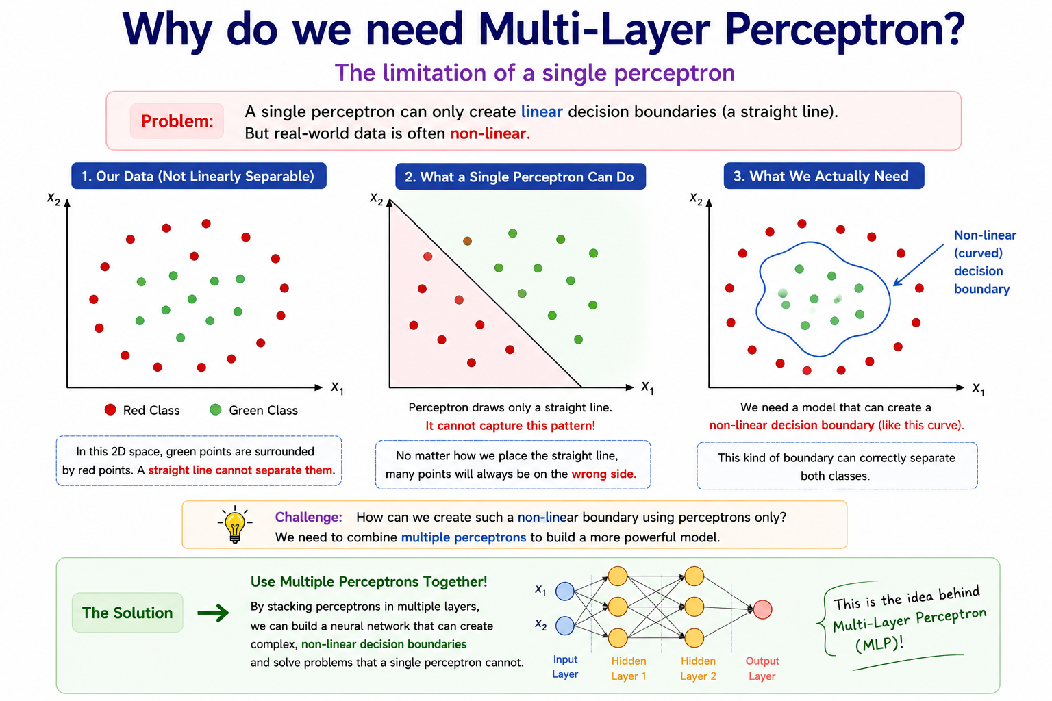
If our goal is to separate these two classes, what kind of boundary would we need?

The answer becomes obvious when we visualize the data. A straight line would not be sufficient because no matter how we position that line, some green points and some red points would always end up on the wrong side. The natural boundary for this dataset is not a line at all. Instead, it is a curved shape that encloses the green region while excluding the surrounding red points.

This is exactly where the perceptron encounters its biggest limitation.

Why the Perceptron Fails

At this point, it is tempting to assume that the perceptron simply needs more training. Perhaps the algorithm has not found the correct weights yet. Maybe increasing the number of iterations or adjusting the learning rate will eventually produce the desired boundary.

Unfortunately, that is not the case.

The problem is not related to training. The problem is related to the model itself. A perceptron is mathematically designed to create linear decision boundaries. Regardless of how long we train it or how carefully we tune its parameters, the final result will always be a straight line. This distinction is extremely important because it helps us understand the difference between a training problem and a model limitation. Training problems can often be solved by providing more data, running additional iterations, or choosing better hyperparameters. Model limitations are much more fundamental. They arise because the model lacks the capacity to represent the desired solution.

In this case, the perceptron simply does not have the ability to create the curved boundary that the dataset requires.

To understand this better, imagine giving a student a ruler and asking them to draw a perfect circle. It does not matter how skilled the student is or how much time they are given. The problem is not their effort. The problem is the tool itself. A ruler is designed to draw straight lines, not circles.

The perceptron suffers from a similar limitation. It is an excellent tool for creating linear boundaries, but the moment a problem requires a non-linear boundary, the perceptron reaches the limits of what it can represent.

##What We Actually Need

Once we recognize the limitation, the next question naturally follows:

If a single perceptron can only draw a straight line, how can we create a curved boundary?

One possible approach would be to design an entirely new algorithm from scratch. However, researchers took a different path. Instead of abandoning the perceptron, they asked a much more interesting question.

What if multiple perceptrons could work together?

Individually, each perceptron can only create a linear boundary. That fact does not change. However, perhaps a collection of perceptrons could cooperate in a way that produces far more sophisticated behavior.

To understand this idea, think about how a polygon is constructed. A single line segment cannot create a closed shape. Yet when many line segments are combined together, they can approximate increasingly complex boundaries. With enough segments, the resulting shape can begin to resemble a curve.

The same intuition applies here.

A single perceptron creates one linear boundary. Multiple perceptrons create multiple linear boundaries. When these boundaries are combined intelligently, they can approximate regions that are impossible for a single perceptron to represent.

This observation forms the foundation of one of the most important ideas in deep learning.

Moving from Step Functions to Probabilities

Before we explore the idea of combining perceptrons, we need to make one small adjustment to our perceptron model.

So far, we have often discussed perceptrons as classifiers that produce discrete outputs such as 0 or 1. While this explanation is useful for understanding the basic concept, modern machine learning models frequently use a sigmoid activation function instead of a hard step function.

As a result, the perceptron no longer outputs only two possible values. Instead, it produces a probability between 0 and 1.

Suppose we are building a model that predicts whether a student will be placed during campus recruitment based on two features:

• CGPA
• IQ

After training, the perceptron learns a set of weights and a bias. Using those values, it computes:

$$z=w_1​x_1​+w_2​x_2​+b$$

The value of $z$ is then passed through the sigmoid function:

$$\sigma(z) = \frac{1}{1 + e^{-z}}$$

The output is always between 0 and 1.

For example, if the sigmoid function returns 0.8, we can interpret that as an 80% probability that the student will be placed. Similarly, an output of 0.2 indicates a 20% probability of placement.

This seemingly small change is extremely important because it allows us to think of a perceptron not merely as a classifier but as a probability estimator.

Understanding the Decision Boundary

When we plot the data in a two-dimensional space, the perceptron still creates a straight-line decision boundary. An interesting property of this boundary is that every point lying directly on the boundary has a probability of 0.5.

Why?

Because the decision boundary corresponds to:

$$w_1​x_1​+w_2​x_2​+b=0$$

Substituting $z=0$ into the sigmoid function gives:

$$σ(0)=0.5$$

This means every point on the boundary has an equal probability of belonging to either class. As we move away from the boundary, the probabilities gradually change. A student located slightly above the boundary might have a placement probability of 0.6. Moving further away might increase that probability to 0.7, then 0.8, and eventually 0.9. Similarly, moving in the opposite direction decreases the probability toward 0.

This creates a smooth probability landscape across the entire feature space.

Instead of abruptly switching between classes, the model gradually changes its confidence as we move through the data.

An Important Observation

At this point, we should pause and make an important observation. Every perceptron effectively provides us with a new view of the dataset. Given any student, the perceptron produces a probability value.

For example:

Student	Probability of Placement
A	0.90
B	0.75
C	0.40
D	0.10

These probabilities contain useful information about how the perceptron sees the data. Now imagine training a second perceptron on the same dataset. Because the weights are different, this second perceptron will create a different decision boundary and therefore produce a different probability estimate for each student.

For the same student, the two perceptrons might produce:

Student	Perceptron 1	Perceptron 2
A	0.90	0.60
B	0.75	0.80
C	0.40	0.55
D	0.10	0.30

Suddenly, every student is described by two probability values instead of one. This raises an interesting possibility.

What if we combine these probabilities?

Combining Multiple Perceptrons

Suppose we train two different perceptrons on the same dataset. The first perceptron learns one linear decision boundary. The second perceptron learns another linear decision boundary. Individually, neither perceptron can solve the non-linear problem. However, their outputs contain different information about the data. Instead of using either perceptron directly, we can combine their outputs.

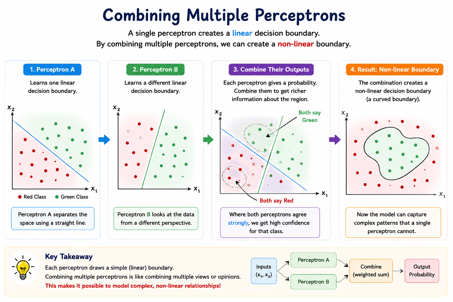
For a particular student:

$$P1​=0.7 \\ P2​=0.8$$

A simple approach would be to add them:

$$P1​+P2​=1.5$$

Unfortunately, 1.5 is not a valid probability because probabilities must lie between 0 and 1. To convert the result back into a probability, we can pass the combined value through another sigmoid function.

$$σ(P1​+P2​)$$

The output again falls between 0 and 1. What we have created here is something entirely new. Instead of directly using the original features, we are using the outputs of existing perceptrons as inputs to another model.

This idea forms the foundation of Multi-Layer Perceptrons.

Giving Different Importance to Different Perceptrons

In practice, not all perceptrons contribute equally. One perceptron may capture a particularly useful pattern, while another may be less informative. Therefore, rather than simply adding the outputs, we assign weights to them.

The combined value becomes:

$$z=w_1​P_1​+w_2​P_2​+b$$

Notice how familiar this equation looks. It is exactly the same weighted-sum equation we saw earlier. The only difference is that the inputs are no longer CGPA and IQ. The inputs are now the outputs of other perceptrons.

After computing $z$, we once again apply the sigmoid function:

$$Output=σ(z)$$

This produces a new probability. At this point, we have essentially built a perceptron whose inputs come from other perceptrons.

That is a remarkable idea because it means perceptrons can be stacked on top of each other.

The Birth of the Multi-Layer Perceptron

Once we view the problem in this way, the structure of a Multi-Layer Perceptron emerges naturally. The first set of perceptrons receives the original input features such as CGPA and IQ.

These perceptrons produce probability outputs. Those outputs are then fed into another perceptron, which combines them to produce a final prediction.

The output of one perceptron has become the input to another perceptron. Instead of a single classifier, we now have a network of interconnected perceptrons. This network is what we call a Multi-Layer Perceptron (MLP).

Introducing Layers

To make these networks easier to understand, we organize the neurons into layers.

The original features form the Input Layer.

The perceptrons that process those features form a Hidden Layer.

The final perceptron that produces the prediction forms the Output Layer.

The hidden layer receives its name because it is not directly visible in the input or output. It exists solely to transform information before passing it forward. Although the architecture appears simple, this additional layer dramatically increases the expressive power of the network.

A single perceptron creates one linear decision boundary. Multiple perceptrons working together can create far more complex decision boundaries, allowing the network to capture patterns that were previously impossible to represent.