Introduction to Perceptron

Perceptron is considered one of the most important foundational concepts in Deep Learning and Artificial Neural Networks. Although modern deep learning systems contain extremely complex neural network architectures with millions or even billions of parameters, the core idea behind many of these systems can still be traced back to the simple perceptron model.

A perceptron is often called the fundamental building block of Artificial Neural Networks because it introduces the basic mechanism through which neural networks receive inputs, process information, learn patterns, and generate predictions.

What is a Perceptron?

A perceptron is a Machine Learning algorithm used mainly for supervised learning and binary classification problems. Just like algorithms such as Linear Regression, Logistic Regression, or Support Vector Machines, the perceptron is also a mathematical learning model capable of making predictions from data.

A simple definition of a perceptron is:

A perceptron is a mathematical model and learning algorithm that takes multiple inputs, processes them using weights and bias, and produces an output prediction.

The perceptron became extremely important in Deep Learning because its design closely resembles the basic idea of how neurons process information inside biological nervous systems. Although a perceptron is much simpler than an actual biological neuron, the inspiration behind the design helped researchers build larger neural networks later.

A perceptron can also be viewed as:

• a Machine Learning algorithm
• a mathematical model
• a mathematical function

All three interpretations are correct depending on the context in which it is being discussed.

Basic Structure of a Perceptron

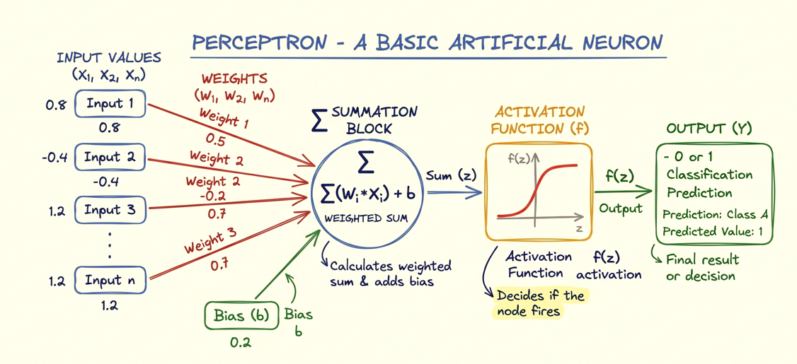
A perceptron consists of several important components working together to process input data and generate predictions.

The main components are:

• Input values
• Weights
• Bias
• Summation block
• Activation function
• Output

The perceptron receives inputs from the outside world. These inputs are usually represented as:

$$x_1,x_2,x_3 \dots x_n$$

Each input is associated with a numerical weight:

$$w_1,w_2,w_3 \dots w_n$$

The perceptron multiplies each input with its corresponding weight and then performs summation.

The mathematical expression becomes:

$$z = w_1x_1 + w_2x_2 + \dots + w_nx_n + b$$

Here:

• $x$ values are inputs
• $w$ values are weights
• $b$ represents bias
• $z$ is the intermediate computed value

The value $z$ is then passed into an activation function which produces the final output.

Understanding Inputs, Weights, and Bias

The inputs represent the features of the data.

Suppose we are building a model that predicts whether a student will get placement in college. The inputs could be:

IQ score CGPA Resume score

If we use only IQ and CGPA, then:

$$x_1 = IQ \\ x_2 = CGPA$$

However, inputs alone are not enough. The perceptron also needs to understand how important each feature is. This importance is represented through weights. A higher weight means that the corresponding feature has greater influence on the prediction.

For example, if:

$$w_1 = 2$$

and

$$w_2 = 4$$

then CGPA is contributing more strongly toward the prediction compared to IQ. This gives us an important interpretation:

Weights represent feature importance inside the perceptron model.

The bias term helps shift the decision boundary and improves the flexibility of the model. Without bias, the perceptron would become too restrictive.

The Summation Process

Once inputs and weights are available, the perceptron performs weighted summation.

Suppose:

$$x_1 = 78 \\ x_2 = 7.8 \\ w_1 = 2 \\ w_2 = 4 \\ b = 3$$

Then the perceptron calculates:

$$z=(2×78)+(4×7.8)+3$$

The summation process combines all feature contributions into a single numerical value. This value itself does not yet represent the final prediction. It must first pass through an activation function.

Activation Function in Perceptron

The activation function is one of the most important components of a perceptron. The weighted sum $z$ can become any large positive or negative number depending on inputs and weights. The role of the activation function is to transform this value into a controlled output range.

One of the simplest activation functions used in perceptrons is the Step Function.

The logic is simple:

• If $z≥0$, output becomes 1
• If $z<0$, output becomes 0

Mathematically:

$$f(z)= \left\{ \begin{array}{ll} 1 & \text{if } z \geq 0 \\ 0 & \text{if } z < 0 \end{array} \right.$$

This makes perceptrons suitable for binary classification problems where the output belongs to one of two classes.

For example:

• Placement or No Placement
• Spam or Not Spam
• Fraud or Non-Fraud

Modern neural networks use more advanced activation functions such as:

• ReLU
• Sigmoid
• Tanh
• Softmax

But the perceptron traditionally uses the simple step function.

Training a Perceptron

Like other Machine Learning algorithms, perceptrons also go through a training process.

The primary goal during training is to find optimal values for weights and bias.

The perceptron studies training examples and gradually adjusts these values so that predictions become more accurate.

Suppose we have data containing:

IQ	CGPA	Placement
78	7.8	1
69	5.1	0

The perceptron processes each student record one by one. During training, it compares predicted outputs with actual outputs and updates weights accordingly.

The core objective of training can be summarized as:

Finding the correct weights and bias values that minimize prediction errors.

Once training completes, the perceptron becomes capable of making predictions on unseen data.

Prediction Using Perceptron

After training, the perceptron can be used for prediction.

Suppose a new student has:

• IQ = 100
• CGPA = 5.1

The perceptron substitutes these values into the learned equation:

$$z = w_1x_1 + w_2x_2 + b$$

If the resulting $z$ becomes positive, the activation function may output 1, indicating placement.

If $z$ becomes negative, the activation function may output 0, indicating no placement.

This entire process demonstrates how perceptrons convert input features into classification decisions.

Geometric Interpretation of Perceptron

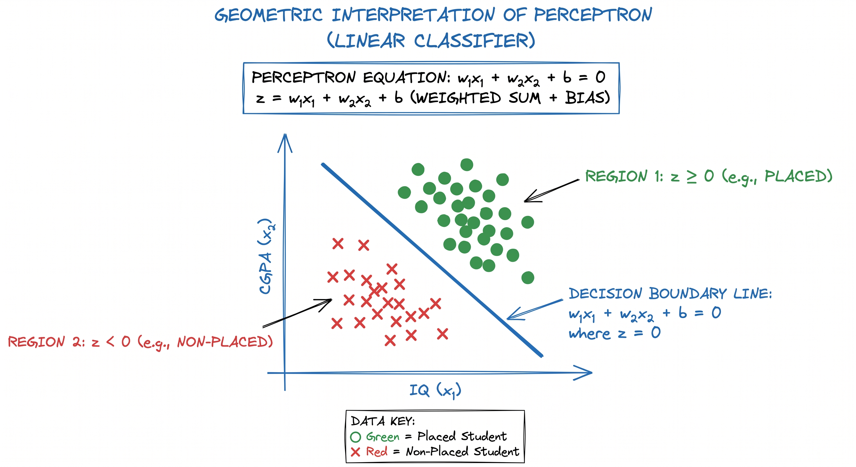
One of the most beautiful aspects of perceptrons is their geometric interpretation.

The perceptron equation:

$$w_1x_1 + w_2x_2 + b = 0$$

represents a line in two-dimensional space.

This means the perceptron is essentially trying to draw a decision boundary that separates two classes.

Suppose we plot students using:

X-axis = IQ Y-axis = CGPA

Placed students may cluster in one region while non-placed students cluster in another.

The perceptron attempts to draw a line separating these regions.

If:

$$z≥0$$

the point belongs to one class.

If:

$$z<0$$

the point belongs to another class.

This is why perceptrons are called binary classifiers. They divide space into two decision regions.

Perceptron in Higher Dimensions

If the dataset contains more than two input features, the perceptron still works similarly. For example:

• IQ
• CGPA
• 12th Marks

Now the equation becomes:

$$z=w_1​x_1​+w_2​x_2​+w_3​x_3​+b$$

In three dimensions, the perceptron creates a plane instead of a line. In even higher dimensions, the perceptron creates what is called a hyperplane.

The central idea remains the same:

The perceptron separates data into regions using a linear decision boundary.

Limitation of Perceptron

The biggest limitation of perceptrons is that they can only solve linearly separable problems. If two classes can be separated using a straight line, plane, or hyperplane, the perceptron performs well. However, if the dataset is highly non-linear, the perceptron fails.

For example, imagine two classes arranged in circular or overlapping patterns where no straight line can separate them properly. In such cases, perceptrons produce poor accuracy.

This limitation eventually led researchers toward Multi-Layer Perceptrons and deeper neural networks capable of learning non-linear relationships.