Changes in Neural Network

In this tutorial, we'll discuss ways to change our neural network.

Increasing the Number of Neurons in a Hidden Layer

Understanding Neural Network Architecture

As we continue exploring Multi-Layer Perceptrons, it is important to understand that the power of a neural network is not determined solely by the presence of hidden layers. Equally important is the architecture of the network itself. In simple terms, the architecture refers to how neurons are organized and connected to one another. Whenever we add new neurons, introduce additional layers, or modify the connections between neurons, we are changing the network's architecture.

So far, most of our examples have used a hidden layer containing only two neurons. This simplified architecture helped us understand how multiple perceptrons can work together to solve problems that a single perceptron cannot. However, real-world datasets are often much more complex, and a hidden layer containing only a few neurons may not always be sufficient to capture the underlying patterns in the data.

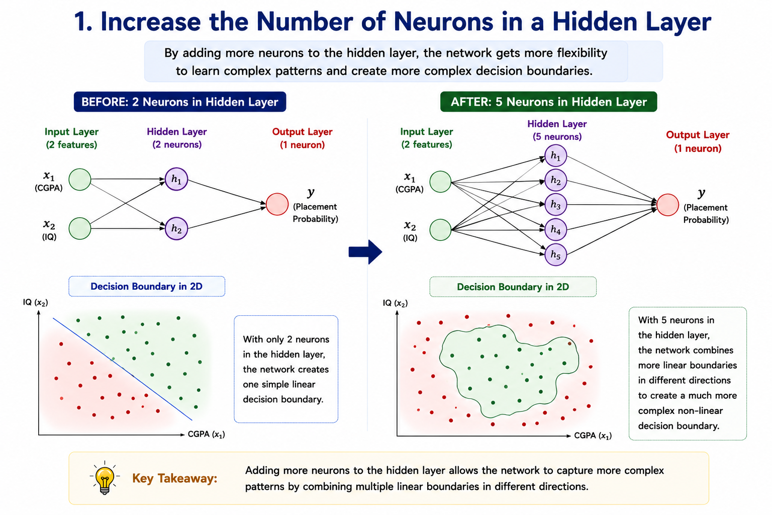
One of the easiest ways to increase the flexibility of a neural network is to add more neurons to its hidden layer.

What Happens When We Add Another Neuron?

Consider a network whose hidden layer contains two neurons. Each neuron receives the same input features, but because they learn different weights and biases, they typically discover different patterns within the data. In other words, each neuron develops its own interpretation of the problem.

Now suppose we add a third neuron to the hidden layer.

Although this new neuron receives exactly the same inputs as the existing neurons, it is free to learn its own set of weights and biases. As training progresses, it may identify a pattern that the other two neurons have not captured. The network therefore gains an additional source of information that can be used when making predictions.

This is an important idea because adding a neuron does not simply increase the amount of computation being performed. Instead, it gives the network another opportunity to learn a useful representation of the data. The change appears small, but its impact on the network's learning capacity can be significant.

Viewing Hidden Neurons as Individual Perceptrons

A useful way to understand the role of hidden neurons is to think of each one as an independent perceptron.

Every hidden neuron performs the familiar sequence of operations:

1. Calculate a weighted sum of its inputs.
2. Add a bias term.
3. Apply an activation function.
4. Produce an output.

Because each neuron learns different parameters, each one effectively creates its own decision boundary. These boundaries are usually different from one another, allowing the neurons to focus on different aspects of the dataset.

If the hidden layer contains two neurons, the network learns two different representations of the data. If the hidden layer contains three neurons, the network learns three representations. As the number of neurons increases, the network gains access to increasingly rich descriptions of the input space.

This additional diversity is what makes larger networks more expressive.

A Geometric Perspective

The effect of adding neurons becomes even easier to understand when viewed geometrically.

Recall that a single perceptron can create only one linear decision boundary. When we combine multiple perceptrons, each hidden neuron contributes its own linear boundary. The output layer then combines the information from all of these boundaries to produce the final prediction.

Imagine trying to approximate a complex curved shape using straight line segments. A single segment provides a very poor approximation. Adding a second segment improves the result slightly. Adding more segments allows the approximation to become increasingly accurate.

Hidden neurons behave in a remarkably similar way.

Each neuron contributes another piece of the final decision boundary. As more neurons are added, the network gains the ability to represent increasingly complex non-linear regions. This is one of the key reasons Multi-Layer Perceptrons can solve problems that are impossible for a single perceptron.

How the Mathematical Computation Changes

Interestingly, the underlying computation remains almost identical when additional neurons are introduced.

Suppose a hidden layer contains two neurons that produce outputs $P1$ and $P2$. The output neuron combines these values using a weighted sum:

$$z=w_1​P_1​+w_2​P_2​+b$$

After applying an activation function, the network produces its final prediction. Now imagine adding a third hidden neuron that produces output $P_3$.

The output layer simply extends the equation:

$$z=w_1​P_1​+w_2​P_2​+w_3​P_3​+b$$

Nothing fundamentally changes about the computation. The network is still combining outputs using a weighted sum. The difference is that it now has access to additional information through $P_3$.

This extra information can help the model identify patterns that were previously difficult or impossible to capture.

Why More Neurons Help with Non-Linear Data

The original motivation for developing Multi-Layer Perceptrons was the inability of a single perceptron to create non-linear decision boundaries. Adding hidden neurons directly addresses this limitation.

Each hidden neuron learns a different transformation of the input data. When these transformations are combined, the network can construct highly flexible decision regions that no individual neuron could create on its own.

As the number of neurons increases, the network becomes capable of representing increasingly complex relationships between inputs and outputs. Datasets that appear highly non-linear can often be modeled successfully because the network has enough neurons to capture the underlying structure.

In essence, every additional neuron provides another building block that can be used to construct the final decision boundary.

Is More Always Better?

At this point, it may seem reasonable to conclude that adding as many neurons as possible will always improve performance. In practice, however, the situation is more nuanced.

A network with too few neurons may lack the capacity required to learn the problem effectively. On the other hand, a network with too many neurons may become unnecessarily complex and begin memorizing the training data instead of learning general patterns.

For this reason, choosing the number of hidden neurons is often a balance between simplicity and expressive power. The goal is not to create the largest possible network but to create a network that has enough capacity to model the complexity of the dataset without becoming excessively complicated.

Adding More Input Nodes

When Do We Need More Input Nodes?

So far, our discussion of Multi-Layer Perceptrons has focused on increasing the network's flexibility by adding more neurons to the hidden layer. While this is one way to make a neural network more expressive, it is not the only way to modify its architecture. Another common architectural change involves increasing the number of nodes in the input layer.

Unlike hidden neurons, input nodes are not added arbitrarily. The number of input nodes is directly determined by the number of input features available in the dataset. In other words, whenever the dataset contains additional information that might help the model make better predictions, the input layer must expand to accommodate those new features.

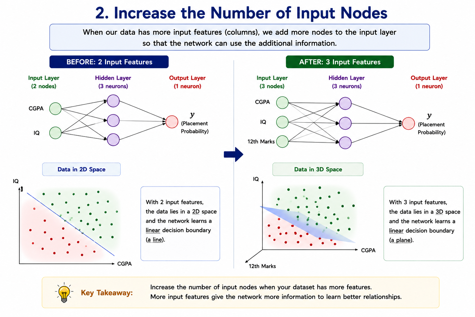
Consider the examples we have used throughout this tutorial series. Suppose we are trying to predict whether a student will get placed during campus recruitment. Initially, we assumed that the prediction depends on only two features:

• CGPA
• IQ

Since there are two input features, the input layer contains two nodes. This simple architecture works because the model has only two pieces of information available for making its prediction.

What Happens When a New Feature Is Added?

Now suppose we discover that another factor plays an important role in placement outcomes:

• 12th Grade Marks

This new feature contains valuable information that was previously unavailable to the network. Since the model must now process three inputs instead of two, the input layer must also grow. Notice that nothing has changed in the hidden layer or the output layer. The only change is that the network now receives an additional input.

This may appear to be a small modification, but it fundamentally changes the space in which the data exists.

Moving from Two Dimensions to Three Dimensions

When a dataset contains only two input features, it can be visualized on a two-dimensional graph.

For example:

• X-axis → CGPA
• Y-axis → IQ

Each student appears as a point in this two-dimensional space. A perceptron operating on this dataset creates a straight-line decision boundary.

We can represent that boundary mathematically as:

$$w_1​x_1​+w_2​x_2​+b=0$$

Geometrically, this equation represents a line. However, once we introduce a third input feature such as 12th Grade Marks, the situation changes.

Now our dataset contains:

• CGPA
• IQ
• 12th Marks

Instead of living in a two-dimensional space, every student now occupies a position in a three-dimensional space.

The axes become:

• X-axis → CGPA
• Y-axis → IQ
• Z-axis → 12th Marks

Every student is now represented by a point in 3D. This additional dimension gives the neural network access to more information and potentially allows it to discover patterns that were invisible in the two-dimensional representation.

How Decision Boundaries Change in Higher Dimensions

When working with two input features, a perceptron creates a line. Once we move to three input features, the perceptron no longer creates a line. Instead, it creates a plane.

The decision boundary becomes:

$$w_1​x_1​+w_2​x_2​+w_3​x_3​+b=0$$

This equation represents a plane in three-dimensional space.

If we train two different perceptrons, each perceptron learns its own plane. Just as two perceptrons previously learned two different lines in a two-dimensional space, they now learn two different planes in a three-dimensional space.

Although visualizing multiple planes is more challenging than visualizing multiple lines, the underlying idea remains exactly the same. Each perceptron learns a different way of dividing the feature space.

Combining Multiple Perceptrons in Three Dimensions

The presence of an additional input feature does not change how the Multi-Layer Perceptron operates internally.

Suppose two hidden neurons receive:

• CGPA
• IQ
• 12th Marks

Each hidden neuron computes its own weighted sum and produces a probability.

For a particular student, the first hidden neuron might produce:

$$P1​=0.7$$

while the second hidden neuron produces:

$$P2​=0.4$$

These probabilities are then combined by the output neuron:

$$z=w_1​P_1​+w_2​P_2​+b$$

After applying the sigmoid function:

$$Output=σ(z)$$

the network generates the final probability of placement.

Notice that the computation is identical to what we saw earlier. The only difference is that the hidden neurons now have access to more information because an additional feature has been provided.

This extra information often enables the network to make more accurate predictions.

What If We Keep Adding More Features?

Suppose we continue adding more input variables:

• CGPA
• IQ
• 12th Marks
• Communication Skills Score
• Coding Assessment Score
• Internship Experience

Every new feature adds another input node. At some point, the dataset may contain dozens or even hundreds of input features.

Geometrically, the decision boundary is no longer a line or a plane. It becomes a hyperplane, which is simply the higher-dimensional generalization of a line and a plane. While humans cannot easily visualize spaces beyond three dimensions, neural networks have no difficulty working in such environments. The underlying mathematics remains exactly the same. A perceptron operating on ten input features creates a hyperplane in ten-dimensional space. A perceptron operating on one hundred input features creates a hyperplane in one hundred-dimensional space.

The concept remains unchanged even though visualization becomes impossible.

Why Additional Input Features Can Improve Performance

The primary reason for adding more input nodes is that additional features often contain useful information about the problem being solved.

Imagine trying to predict a student's placement outcome using only CGPA. The prediction may be reasonably accurate, but it ignores many other factors that influence placement decisions.

Adding IQ introduces more information. Adding 12th Grade Marks introduces even more information. Adding coding scores, internship experience, and communication skills may further improve the model's understanding of the problem. Each new feature provides another perspective on the data, allowing the network to make more informed decisions.

Of course, not every feature is useful. Some features may contain irrelevant or noisy information. However, when a feature genuinely contributes to the prediction task, expanding the input layer allows the neural network to leverage that information.

Adding More Output Nodes

Why Would We Need More Output Nodes?

So far, all the neural network examples we have discussed have shared one common characteristic: the output layer contained only a single neuron. This design made sense because our problems involved binary classification tasks, where the model needed to answer a simple question with only two possible outcomes. For example, we might want to predict whether a student will get placed or not, determine whether an email is spam or not, or classify a transaction as fraudulent or legitimate.

In such scenarios, a single output neuron is sufficient because the model only needs to estimate the probability of one class. If the probability exceeds a certain threshold, we predict one class; otherwise, we predict the other.

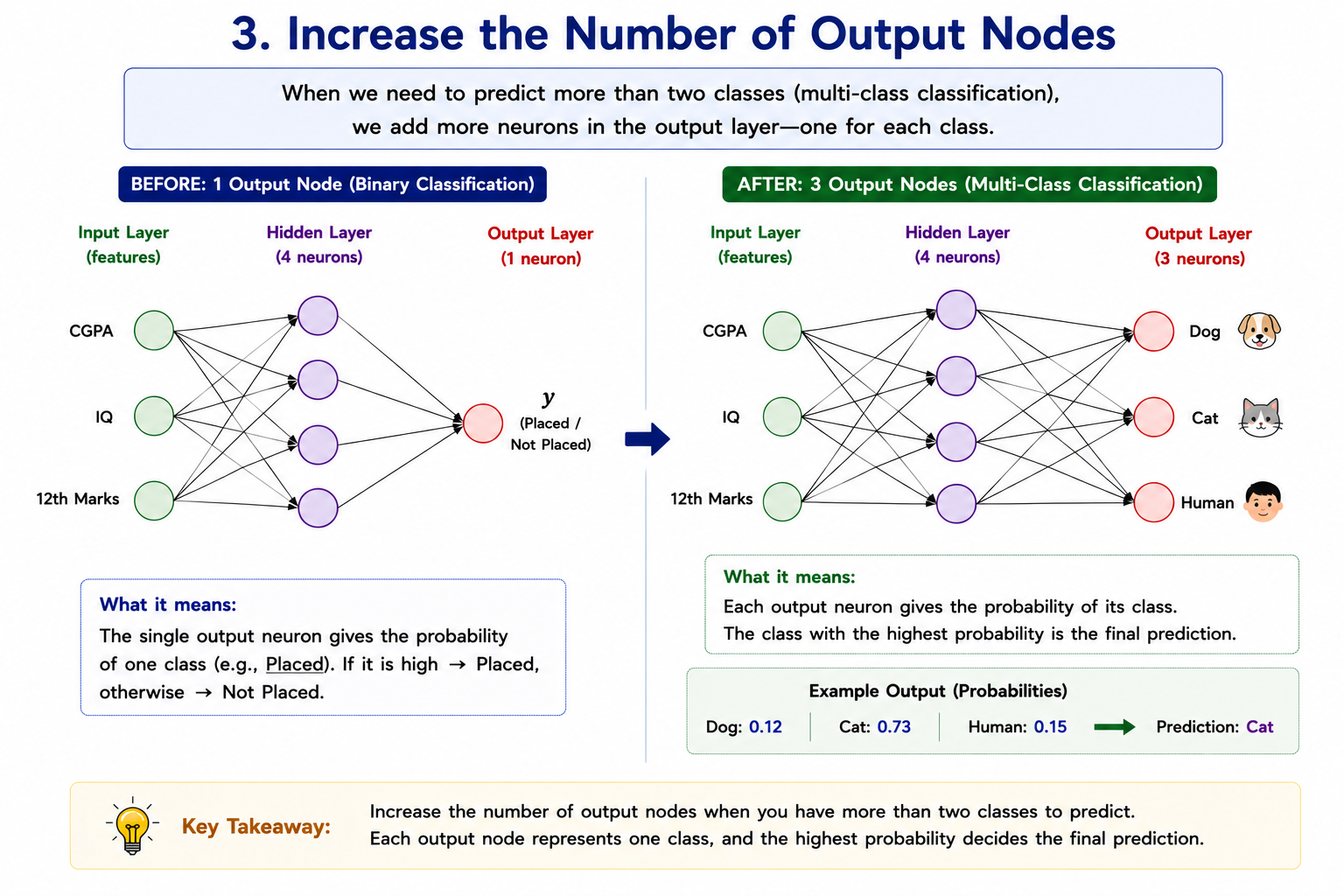
However, many real-world problems are more complex than binary classification. Instead of choosing between two possibilities, the model may need to choose from several categories. When this happens, a single output neuron is no longer enough, and we need to modify the architecture of the network by increasing the number of output nodes.

From Binary Classification to Multi-Class Classification

To understand why multiple output neurons are needed, consider a simple image classification problem.

Suppose we have built a neural network that receives an image as input, and our goal is to identify the object present in that image. Unlike a binary classification problem, the image may belong to one of several categories.

For example, imagine that every image belongs to one of the following classes:

• Dog
• Cat
• Human

Now the network is no longer answering a yes-or-no question. Instead, it must determine which of the three possible categories best describes the image.

A single output neuron cannot naturally represent these three possibilities. Instead, we create a separate output neuron for each class.

How Multiple Output Neurons Work

Suppose an image is passed through the neural network.

After processing the image through all hidden layers, the network reaches the output layer. Instead of producing a single value, it now produces three probability scores:

Class	Probability
Dog	0.85
Cat	0.10
Human	0.05

These values indicate how confident the network is that the image belongs to each category.

In this example, the highest probability corresponds to the Dog class. Therefore, the model predicts that the image contains a dog.

Now consider another image:

Class	Probability
Dog	0.12
Cat	0.80
Human	0.08

Since the Cat neuron produces the highest probability, the network classifies the image as a cat.

The decision-making process is therefore very straightforward:

The output neuron with the highest probability determines the final prediction.

A Geometric Interpretation

The hidden layers of the network continue to perform the same job they always have. They learn useful representations of the input data and extract patterns that help distinguish one class from another.

The difference appears only in the final stage of the network.

In a binary classification problem, the network ultimately decides between two regions of the feature space. With multi-class classification, the network must partition the feature space into multiple regions, one for each class.

For example, if we are classifying images into Dog, Cat, and Human categories, the network must learn boundaries that separate all three groups simultaneously.

Each output neuron contributes to this decision-making process by estimating how strongly the input belongs to its associated class.

As the number of classes increases, the network requires additional output neurons so that every class can have its own probability estimate.

What Changes Mathematically?

The underlying computation remains very similar to what we have already seen.

In a binary classification problem, the output layer may contain a single neuron:

$$z=w_1​h_1​+w_2​h_2​+w_3​h_3​+b$$

which is then passed through an activation function to produce a probability.

When we move to a three-class problem, we simply create three separate output neurons.

The Dog neuron computes:

$$z_{dog}​=w_1​h_1​+w_2​h_2​+w_3​h_3​+b_{dog​}$$

The Cat neuron computes:

$$z_{cat}​=w_1​h_1​+w_2​h_2​+w_3​h_3​+b_{cat}​$$

The Human neuron computes:

$$z_{human}​=w_1​h_1​+w_2​h_2​+w_3​h_3​+b_{human​}$$

Each neuron learns its own weights and bias values, allowing it to specialize in recognizing its corresponding class.

The outputs are then converted into probabilities, allowing the network to determine which class is the most likely.

Does Every Problem Need Multiple Output Nodes?

The answer depends entirely on the nature of the prediction task. If the problem involves only two classes, a single output neuron is usually sufficient.

Examples include:

• Pass or Fail
• Spam or Not Spam
• Fraud or Not Fraud
• Placed or Not Placed

However, when the number of possible classes increases, the output layer must expand accordingly.

Examples include:

• Dog, Cat, Human
• Car, Bus, Bike, Truck
• Apple, Mango, Banana, Orange
• Happy, Sad, Angry, Neutral

In these situations, multiple output neurons provide a natural way to estimate the probability of each class separately.

Why This Architectural Change Is Important

Adding output neurons does not increase the complexity of the hidden representations in the same way that adding hidden neurons does. Instead, it increases the number of categories the network can predict.

Hidden neurons primarily improve the network's ability to learn complex patterns. Output neurons primarily improve the network's ability to represent multiple prediction classes.

This distinction is important because many beginners assume that all neurons serve the same purpose. In reality, neurons in different layers play different roles.

Input nodes represent features.

Hidden neurons learn patterns.

Output neurons represent possible predictions.

By increasing the number of output nodes, we allow the network to handle increasingly sophisticated classification tasks without fundamentally changing how the rest of the network operates.

Adding More Hidden Layers: Deep Neural Networks

From Multi-Layer Perceptrons to Deep Neural Networks

So far, we have explored several ways of modifying a neural network's architecture. We learned that we can increase the number of neurons in a hidden layer, add more input nodes when additional features become available, and increase the number of output nodes when solving multi-class classification problems. All of these modifications make the network more flexible, but there is another architectural change that has had an even greater impact on the field of Artificial Intelligence: increasing the number of hidden layers.

Up to this point, most of our examples have contained only a single hidden layer. The architecture typically looked something like this:

Input Layer
      ↓
Hidden Layer
      ↓
Output Layer

This structure is already capable of learning many non-linear relationships. However, as datasets become more complex, a single hidden layer may not always be sufficient to capture all the underlying patterns. In such situations, we can introduce additional hidden layers, allowing the network to learn increasingly sophisticated representations of the data.

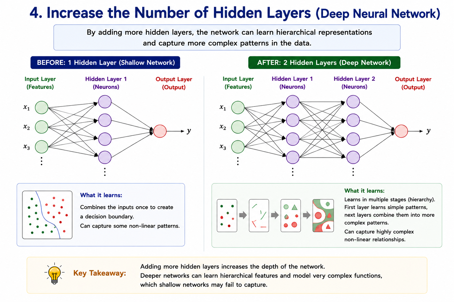
When a neural network contains multiple hidden layers, it is commonly referred to as a Deep Neural Network (DNN). The term deep does not imply anything mysterious; it simply refers to the depth of the network, which is determined by the number of hidden layers it contains.

What Changes When We Add More Hidden Layers?

At first glance, adding another hidden layer may seem similar to adding more neurons. After all, both changes increase the size of the network. However, the two modifications serve different purposes.

When we add more neurons to a hidden layer, we increase the network's ability to learn different patterns at the same level of abstraction. Each neuron learns a slightly different view of the data, and together they create richer decision boundaries.

Adding another hidden layer is different. Instead of simply learning more patterns, the network begins learning patterns of patterns.

To understand this idea, imagine a network trying to recognize handwritten digits. The first hidden layer may learn simple structures such as edges and lines. The second hidden layer can combine those edges and lines into more meaningful shapes. A third hidden layer can combine those shapes into complete digits.

Each layer builds upon the information produced by the previous layer. As we move deeper into the network, the learned representations become increasingly abstract and increasingly useful for solving complex problems.

This hierarchical learning process is one of the primary reasons deep neural networks have become so successful.

Learning More Complex Relationships

Consider the non-linear datasets we discussed earlier in this tutorial series. A single perceptron can only create a straight-line decision boundary. A Multi-Layer Perceptron with one hidden layer can combine multiple linear boundaries and create more complex non-linear regions.

But what happens when the dataset contains patterns that are even more complicated?

Imagine a dataset where the classes are intertwined in highly irregular ways. The relationships between the input features may involve multiple levels of interaction, making the decision boundary extremely complex.

In such cases, a shallow network may struggle because it lacks sufficient representational power.

By adding more hidden layers, we allow the network to learn increasingly sophisticated transformations of the input data. The first hidden layer may capture simple patterns. The next layer can combine those patterns into more meaningful structures. Subsequent layers can build even more advanced representations.

The result is a network capable of modeling relationships that would be extremely difficult or impossible for a shallow architecture to represent efficiently.

Understanding Feature Hierarchies

One of the most important concepts in deep learning is the idea of a feature hierarchy.

Every hidden layer receives information from the previous layer and transforms it into a new representation. As information flows deeper into the network, the representations become more abstract.

For example, consider an image classification problem.

The first hidden layer may learn:

• Edges
• Corners
• Simple textures

The second hidden layer may combine those features to detect:

• Eyes
• Ears
• Noses

The third hidden layer may combine those structures to recognize:

• Faces
• Animals
• Objects

Notice how each layer builds upon the work of the previous layer.

The network is not explicitly programmed to learn these concepts. Instead, it discovers them automatically during training.

This ability to learn hierarchical representations is one of the defining characteristics of deep neural networks.

Why Deep Networks Are So Powerful

The power of deep neural networks comes from their ability to repeatedly transform data through multiple layers.

Each layer performs a non-linear transformation of the information it receives. The output of one layer becomes the input to the next layer, allowing increasingly complex relationships to emerge.

A useful way to think about this process is as a sequence of feature transformations.

The first layer transforms the raw input into a set of useful features.

The second layer transforms those features into higher-level features.

The third layer transforms those higher-level features into even more meaningful representations.

As more layers are added, the network gains the ability to model highly intricate relationships within the data.

This is why deep learning systems can solve problems such as:

• Image recognition
• Speech recognition
• Language translation
• Object detection
• Text generation

These tasks involve patterns that are far too complex to be captured by simple linear models.

Neural Networks as Universal Function Approximators

The increasing power of deep neural networks leads us to a remarkable idea known as the Universal Approximation Principle.

The core idea is surprisingly simple.

Any real-world problem can be viewed as an unknown mathematical function that maps inputs to outputs. The goal of machine learning is to discover that function using examples.

Researchers have shown that neural networks are capable of approximating extremely complex functions. Given sufficient neurons, sufficient hidden layers, enough training data, and enough training time, a neural network can learn relationships that are arbitrarily close to the underlying function generating the data.

This does not mean the network magically understands the problem. Rather, it means that the architecture is flexible enough to represent an enormous variety of mathematical relationships.

This property is one of the reasons neural networks are often described as universal function approximators.

In practical terms, it means that neural networks can be applied to a vast range of problems without requiring a completely different mathematical model for each task.

Does This Mean We Can Keep Adding Layers Forever?

At this point, it might seem that the solution to every machine learning problem is simply to keep adding more hidden layers.

In theory, deeper networks can represent more complex functions. In practice, however, increasing depth introduces new challenges.

As the number of layers grows:

• Training becomes slower.
• More computational resources are required.
• The number of trainable parameters increases.
• Optimization becomes more difficult.
• Additional techniques are often needed to train the network effectively.

Therefore, while deeper networks are generally more powerful, they also become more demanding to train.

The goal is not to create the deepest possible network but to create a network with enough depth to capture the complexity of the problem being solved.